Project - Kalman Filter

My presentation slides

What is Kalma Filter

The Kalman Filter is a mathematical algorithm used for estimating and predicting the state of a dynamic system, particularly in the presence of noisy or uncertain data. It consist of five equations.

Predict State

---

Predict State:
$\hat{x}_{n+1,n} = F\hat{x}_{n,n} + Gu_n + \omega_n$
Predict Noise:
$\hat{P}_{n+1,n} = F\hat{P}_{n,n}F^T + Q$

Update State

---

Kalman Gain:
$K_n = P_{n, n-1}H^T(HP_{n,n-1}H^T + R_n)^{-1}$
Update State:
$\hat{x}_{n,n} = \hat{x}_{n,n-1} + K_n(z_n-H\hat{x}_{n,n-1})$
Update Noise:
$P_{n,n} = (I-K_nH)P_{n,n-1}(I-K_nH)^T + K_nR_nK_n^T$

State Extrapolation Equation

$\hat{x}_{n+1,n} = F\hat{x}_{n,n} + Gu_n + \omega_n$

Item	Mean
$\hat{x}_{n+1,n}$	predicted system state vector at time step $n+1$
$\hat{x}_{n,n}$	estimated system state vector at time step $n$
$u_n$	a control variable or input variable - a measurable (deterministic) input to the system
$w_n$	a process noise or disturbance - an unmeasurable input that affects the state
$F$	a state transition matrix
$G$	a control matrix or input transition matrix (mapping control to state variables)

Prediction

1. $\hat x^- = F\hat x_{t-1} + Bu_{t-1}$
2. $P_t^- = FP_{t-1}F^T+Q$

Update

1. $\hat x_t = \hat x_t^- + K_t(Z_t - H\hat x_t^-)$

2. $K_t = P_t^-H^T(HP_t^-H^T+R)^{-1}$

3. $P_t=(I - K_tH)P_t^-$

4. Get the best estimation using the measurment.

5. Kalman gamin.

6. Update the noise distribution of best estimates.

$K_t$: Kalman gain
$R$: Observation covariance

Important basic concepts

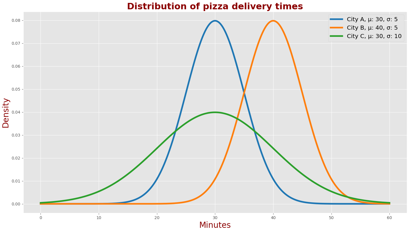
1. Mean $\mu = \frac{1}{N}\displaystyle\sum_{n=1}^{N}V_n$
2. Expectation: The mean of multiple measurements， similar with mean
3. Variance: $\sigma^2 = \frac{1}{N} \displaystyle\sum_{n=1}^{N}(V_n-\mu)^2$
4. Standard Variance: $\sigma$
5. Normal Distribution (All called Gaussian Distribution)
   $f(x; \mu, \sigma^2) = \frac{1}{\sqrt{2\pi\sigma^2}}e^{\frac{-(x-\mu)^2}{2\sigma^2}}$
   
   Typically, measurement errors are normally distributed. The Kalman filter assumes that the measurement errors have a normal distribution.
6. Estimation: An estimate of the hidden state of the system.
7. Accuracy: Describes how close a measured value is to the true value.
8. Precision: Describes the deviation distribution of a series of measured values relative to the same true value

   Info

   High-precision systems have measurements with very low variance (i.e., low uncertainty), while low-precision systems have high variance (i.e., high uncertainty).

Info

Typically, measurement errors are normally distributed. The Kalman filter assumes that the measurement errors have a normal distribution.

Example

How to measure a gold

How to weight a $x$ gold.

Measure a gold

Info

item	mean
$x$	The true weight of the gold.
$z_n$	The measurement of gold.
$\hat{x}_{n,n}$	The estimation of $x$ using the measurement at n moment
$\hat{x}_{n+1,n}$	It is the prediction of the future state (time $n+1$) at time $n$, recorded as $x_{n+1,n}$, or extrapolation.
$\hat{x}_{n−1,n−1}$	The estimated value of $x$ at time $n−1$, using the measured value $z_{n−1}$ at time $n−1$.
$\hat{x}_{n,n-1}$	Apriori estimate - a prediction of the system state at time n at time n−1 (Annotation: for the $n^{th}$ time, $x_{n,n−1}$ is a priori estimate, $x_{n+1, n}$ is prediction)

In order to estimate $x_{n,n}$, we need to store all historical measurements, which is very expensive on memory. And every time a new measurement value is obtained, the calculation needs to be completely restarted from the first measurement, which also consumes a huge amount of CPU computing power.
A more realistic consideration is that it is best to only store the estimated value $x_{n−1,n−1}$ of the previous moment, and simply update it after new measurements are completed.

Formula	Meaning
$\hat x_{n,n} = \frac{1}{n}\sum_{i=1}^{n}(Z_i)$	The mean of measurement
$= \frac{1}{n}(\sum_{i=1}^{n-1}(Z_i)+ Z_n)$
$= \frac{1}{n}\sum_{i=1}^{n-1}(Z_i)+ \frac{1}{n}Z_n$
$= \frac{1}{n}\frac{n-1}{n-1}\sum_{i=1}^{n-1}(Z_i)+ \frac{1}{n}Z_n$
$= \frac{n-1}{n}\textcolor{orange}{\frac{1}{n-1}\sum_{i=1}^{n-1}(Z_i)}+ \frac{1}{n}Z_n)$	The orange item is the estimation at time n-1
$= \frac{n-1}{n}\textcolor{orange}{\hat x_{n-1, n-1}}+ \frac{1}{n}Z_n)$
$= \hat x_{n-1, n-1} - \frac{1}{n}\hat x_{n-1, n-1}+ \frac{1}{n}Z_n$
$= \hat x_{n-1, n-1} - \frac{1}{n}(\hat x_{n-1, n-1} + Z_n)$	The final formula

The final formula is the status update equation. One of five equations of Kalman filter.

Track constant velocity car in one-dimension

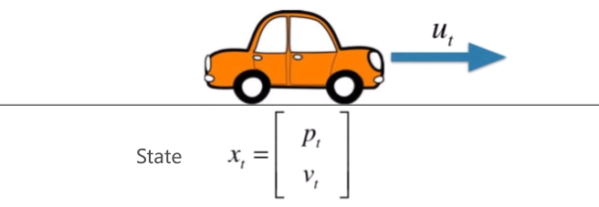
Accelerate: $v= \frac{\Delta x}{\Delta t}$
Velocity prediction: $x_{n+1} = x_n + \Delta t*v_n$
Velocity update: $v_{n+1} = v_n$

How to track a Car

Alt text

Position	$p_t = p_{t-1} + v_{t-1}\Delta t + u_t\frac{\Delta t^2}{2}$
Speed	$v_t = v_{t-1} + u_t\Delta t$

The two formula could be transfored into

$\begin{bmatrix} p_t\\ v_t \end{bmatrix} = \begin{bmatrix} 1 & \Delta t\\ 0 & 1 \end{bmatrix}\begin{bmatrix} p_{t-1}\\ v_{t-1} \end{bmatrix} + \begin{bmatrix} \frac{\Delta t^2}{2}\\ \Delta t \end{bmatrix}u_t$

$F_t = \begin{bmatrix} 1 & \Delta t\\ 0 & 1 \end{bmatrix}, B_t = \begin{bmatrix} \frac{\Delta t^2}{2}\\ \Delta t \end{bmatrix}u_t$

Then the formulas could be transformed into
$\hat x^- = F\hat x_{t-1} + Bu_{t-1}$

How to track a plane

If we want to track a plane, how to do it.
The state will be $x = x_0 + v_0\Delta t + \frac{1}{2}a\Delta t^2$

Info

Item	Mean
$x$	The position of an airplan
$x_0$	The initial postion
$v_0$	The initial speed
$a$	The acceleration
$\Delta t$	Sample period

Predict State

---

Predict State:
$\hat{x}_{n+1,n} = F\hat{x}_{n,n} + Gu_n + \omega_n$
Predict Noise:
$\hat{P}_{n+1,n} = F\hat{P}_{n,n}F^T + Q$

Update States

---

Kalman Gain:
$K_n = P_{n, n-1}H^T(HP_{n,n-1}H^T + R_n)^{-1}$
Update State:
$\hat{x}_{n,n} = \hat{x}_{n,n-1} + K_n(z_n-H\hat{x}_{n,n-1})$
Update Noise:
$P_{n,n} = (I-K_nH)P_{n,n-1}(I-K_nH)^T + K_nR_nK_n^T$

---

1. State Extrapolation equation

$\hat{x}_{n+1,n} = F\hat{x}_{n,n} + Gu_n + \omega_n$

Item	Mean
$\hat{x}_{n+1, n}$	Predicted system state vector at time step $n+1$
$\hat{x}_{n, n}$	Estimated system state vector at time step $n$
$u_n$	Control variable or input variable - a measurable (deterministic) input to the system
$\omega_n$	process noise or disturbance - an unmeasurable input that affects the state
$F$	state transition matrix
$G$	control matrix or input transition matrix (mapping control to state variables)

Airplane without control input

Consider an airplane moving in three-dimensional space with constant acceleration.

The state vector $\hat{x}_n = \begin{bmatrix} x \\ y \\ y \\ \dot{x} \\ \dot{y} \\ \dot{z} \\ \ddot{x} \\ \ddot{y} \\ \ddot{z} \end{bmatrix}$

The state transition matrix $F = \begin{bmatrix} 1 & 0 & 0 &\Delta{t} & 0 & 0 & 0.5\Delta{t^2} & 0 & 0\\ 0 & 1 & 0 & 0 &\Delta{t} & 0 & 0 & 0.5\Delta{t^2} & 0\\ 0 & 0 & 1 & 0 & 0 &\Delta{t} & 0 & 0 & 0.5\Delta{t^2}\\ 0 & 0 & 0 & 1 & 0 & 0 &\Delta{t} & 0 & 0\\ 0 & 0 & 0 & 0 & 1 & 0 & 0 &\Delta{t} & 0\\ 0 & 0 & 0 & 0 & 0 & 1 & 0 & 0 &\Delta{t}\\ 0 & 0 & 0 & 0 & 0 & 0 & 1 & 0 & 0\\ 0 & 0 & 0 & 0 & 0 & 0 & 0 & 1 & 0\\ 0 & 0 & 0 & 0 & 0 & 0 & 0 & 0 & 1 \end{bmatrix}$

The state extrapolation equation is:
$\begin{bmatrix} 1 & 0 & 0 &\Delta{t} & 0 & 0 & 0.5\Delta{t^2} & 0 & 0\\ 0 & 1 & 0 & 0 &\Delta{t} & 0 & 0 & 0.5\Delta{t^2} & 0\\ 0 & 0 & 1 & 0 & 0 &\Delta{t} & 0 & 0 & 0.5\Delta{t^2}\\ 0 & 0 & 0 & 1 & 0 & 0 &\Delta{t} & 0 & 0\\ 0 & 0 & 0 & 0 & 1 & 0 & 0 &\Delta{t} & 0\\ 0 & 0 & 0 & 0 & 0 & 1 & 0 & 0 &\Delta{t}\\ 0 & 0 & 0 & 0 & 0 & 0 & 1 & 0 & 0\\ 0 & 0 & 0 & 0 & 0 & 0 & 0 & 1 & 0\\ 0 & 0 & 0 & 0 & 0 & 0 & 0 & 0 & 1 \end{bmatrix} \begin{bmatrix} x_{(n-1)} \\ y_{(n-1)} \\ z_{(n-1)} \\ \dot{x}_{ (n-1)} \\ \dot{y}_{ (n-1)} \\ \dot{z}_{ (n-1)} \\ \ddot{x}_{(n-1)} \\ \ddot{y}_{(n-1)} \\ \ddot{z}_{(n-1)} \end{bmatrix} \rightarrow \begin{cases} x_n = x_{n-1} + v_{n-1}\Delta t + \frac{1}{2}a_{n-1}\Delta t^2\\ y_n = y_{n-1} + v_{n-1}\Delta t + \frac{1}{2}a_{n-1}\Delta t^2\\ z_n = z_{n-1} + v_{n-1}\Delta t + \frac{1}{2}a_{n-1}\Delta t^2\\ \dot{x}_n = \dot{x}_{n-1} + \ddot{x}_{n-1}\Delta{t}\\ \dot{y}_n = \dot{y}_{n-1} + \ddot{7}_{n-1}\Delta{t}\\ \dot{z}_n = \dot{z}_{n-1} + \ddot{z}_{n-1}\Delta{t}\\ \ddot{x}_{n} = \ddot{x}_{n-1}\\ \ddot{y}_{n} = \ddot{y}_{n-1}\\ \ddot{z}_{n} = \ddot{z}_{n-1} \end{cases}$

Airplane with control input

The state vector $\hat{x}_n$ that describes the estimated airplane position and velocity in a cartesian coordinate system like below.

$\hat{x}_n = \begin{cases} \hat{x}_n\\ \hat{y}_n\\ \hat{z}_n\\ \hat{\dot{x}}_n\\ \hat{\dot{y}}_n\\ \hat{\dot{z}}_n \end{cases}$

The control vector $u_n$ that describes the measured airplane acceleration in a cartesian coordinate system
$u_n = \begin{bmatrix} \ddot{x}_n\\ \ddot{y}_n\\ \ddot{z}_n \end{bmatrix}$

The state transition matrix: $F = \begin{bmatrix} 1 & 0 & 0 &\Delta{t} & 0 & 0\\ 0 & 1 & 0 & 0 &\Delta{t} & 0\\ 0 & 0 & 1 & 0 & 0 &\Delta{t}\\ 0 & 0 & 0 & 1 & 0 & 0\\ 0 & 0 & 0 & 0 & 1 & 0\\ 0 & 0 & 0 & 0 & 0 & 1 \end{bmatrix}$

The control matrix: $G = \begin{bmatrix} 0.5\Delta{t^2} & 0 & 0\\ 0 & 0.5\Delta{t^2} & 0\\ 0 & 0 & 0.5\Delta{t^2}\\ \Delta{t} & 0 & 0\\ 0 &\Delta{t} & 0\\ 0 & 0 &\Delta{t} \end{bmatrix}$

Thus the state prediction formula $\hat{x}_{n+1,n} = F\hat{x}_{n,n} + Gu_n$ will transform like below.

$\hat{x}_{n+1,n} = \begin{bmatrix} x_{(n+1,n)} \\ y_{(n+1,n)} \\ z_{(n+1,n)} \\ \dot{x}_{(n+1,n)} \\ \dot{y}_{(n+1,n)} \\ \dot{z}_{(n+1,n)} \end{bmatrix} = \begin{bmatrix} 1 & 0 & 0 &\Delta{t} & 0 & 0\\ 0 & 1 & 0 & 0 &\Delta{t} & 0\\ 0 & 0 & 1 & 0 & 0 &\Delta{t}\\ 0 & 0 & 0 & 1 & 0 & 0\\ 0 & 0 & 0 & 0 & 1 & 0\\ 0 & 0 & 0 & 0 & 0 & 1 \end{bmatrix}\begin{bmatrix} x_{(n,n)} \\ y_{(n,n)} \\ z_{(n,n)} \\ \dot{x}_{(n,n)} \\ \dot{y}_{(n,n)} \\ \dot{z}_{(n,n)} \end{bmatrix} + \begin{bmatrix} 0.5\Delta{t^2} & 0 & 0\\ 0 & 0.5\Delta{t^2} & 0\\ 0 & 0 & 0.5\Delta{t^2}\\ \Delta{t} & 0 & 0\\ 0 &\Delta{t} & 0\\ 0 & 0 &\Delta{t} \end{bmatrix}\begin{bmatrix} \ddot{x}_n\\ \ddot{y}_n\\ \ddot{z}_n \end{bmatrix}$

2. Covariance extrapolation equation

$P_{(n+1, n)} = FP_{n,n}F^T + Q$

Item	Mean
$P_{n,n}$	The squared uncertainty of an estimate (covariance matrix) of the current state
$P_{n,n}$	The squared uncertainty of a prediction (covariance matrix) for the next state
$F$	The state transition matrix that we derived in the "Modeling linear dynamic systems" section
$Q$	The process noise matrix

Estimate covariance without process noise

Assume that the process noise is equal to zero (Q=0)

$P_{(n+1, n)} = FP_{n,n}F^T$

Becuase of: $P = COV(x) = E((x-\mu_x)(x-\mu_x)^T)$

Thus, $P_{n,n} = E((\hat{x}_{n,n} - \mu_{x_{n,n}})(\hat{x}_{n,n} - \mu_{x_{n,n}})^T)$

Because of the state prediction like
$\hat{x}_{n+1, n} = F\hat{x}_{n, n} + G\hat{u}_{n,n}$

Therefore:

$$\begin{equation} \begin{split} P_{n+1, n} =& E((\hat{x}_{n+1,n} -\mu_{x_{n+1,n}})(\hat{x}_{n+1,n} -\mu_{x_{n+1,n}})^T)\\ \dArr \\ =&E((F\hat{x}_{n,n} + G\hat{u}_{n,n}-F\mu_{x_{n,n}} - G\hat{u}_{n,n})(F\hat{x}_{n,n} + G\hat{u}_{n,n} + G\hat{u}_{n,n}-F\mu_{x_{n,n}}-G\hat{u}_{n,n})^T)\\ \dArr \\ =&E(F(\hat{x}_{n,n} -\mu_{x_{n,n}})(F(\hat{x}_{n,n} -\mu_{x_{n,n}}))^T) \\ \dArr \\ =& E(F(\hat{x}_{n,n} - \mu_{x_{n,n}})(\hat{x}_{n,n} - \mu_{x_{n,n}})^TF^T) \\ \dArr \\ =& FE((\hat{x}_{n,n} - \mu_{x_{n,n}})(\hat{x}_{n,n} - \mu_{x_{n,n}})^T) \\ \dArr \\ =& FP_{n,n}F^T \end{split} \end{equation}$$

Estimate covariance with process noise $Q$

Becuase of process noise $\omega$ exists, thus $\hat{x}_{n+1,n} + F\hat{x}_{n,n} + G\hat{u}_{n,n} + \omega_n$

Where $\omega_n$ is the process noise at the time step $n$.

We've seen that the process noise variance has a critical influence on the Kalman Filter performance. Too small $q$ causes a lag error (see Example 7).. If the $q$ value is too high, the Kalman Filter follows the measurements (see Example 8) and produces noisy estimations.

The process noise can be independent between different state variables. In this case, the process noise covariance matrix $\bar Q$ is a diagonal matrix:

$Q = \begin{bmatrix} q_{11} & 0 & \ldots & 0 \\ 0 & q_{22} & \ldots & 0 \\ \vdots & \vdots & \ddots & \vdots \\ 0 & 0 & ... & q_{kk} \end{bmatrix}$

The process noise can also be dependent. For example, the constant velocity model assumes zero acceleration ($a=0$). However, a random variance in acceleration $σ2a$ causes a variance in velocity and position. In this case, the process noise is correlated with the state variables.

There are two models for the environmental process noise.

• Discrete noise model
• Continuous noise model

3. Measurement equation

The generalized measurement
$z_n = Hx_n + v_n$

Item	Mean	Dimension
$z_n$	measurement vector	$n_x \times 1$
$x_n$	true system state (hidden state)	$n_z \times 1$
$v_n$	Random noise vector	$n_z \times n_x$
$H$	an observation matrix	$n_z \times 1$

In many cases, the measured value is not the desired system state. For example, a digital electric thermometer measures an electric current, while the system state is the temperature. There is a need for a transformation of the system state (input) to the measurement (output).

The purpose of the observation matrix $H$ is to convert the system state into outputs using linear transformations.

Scaling
A range meter sends a signal toward a destination and receives a reflected echo. The measurement is the time delay between the transmission and reception of the signal. The system state is the range.

In this case, we need to perform a scaling:

$z_n = [\frac{2}{c}]x_n + v_n$

Item	Desc
$H$	$[\frac{2}{c}]$
$c$	The speed of light
$x_n$	The range
$z_n$	The measured time delay

State Selection
Sometimes certain states are measured while others are not. For example, the first, third, and fifth states of a five-dimensional state vector are measurable, while the second and fourth states are not measurable:

$z_n = Hx_n + v_n = \begin{bmatrix} 1 & 0 & 0 & 0 & 0\\ 0 & 1 & 0 & 0 & 0\\ 0 & 0 & 1 & 0 & 0 \end{bmatrix}\begin{bmatrix} x_1\\ x_2\\ x_3\\ x_4\\ x_5 \end{bmatrix} + v_n = \begin{bmatrix} x_1\\ x_3\\ x_5 \end{bmatrix} + v_n$

Combination of States
Sometimes some combination of states can be measured instead of each separate state. For example, maybe the lengths of the sides of a triangle are the states, and only the total perimeter can be measured:

$z_n = Hx_n + v_n = \begin{bmatrix} 1 & 1 & 1 \end{bmatrix}\begin{bmatrix} x_1\\ x_2\\ x_3 \end{bmatrix} + v_n = (x_1 + x_2 + x_3)+ v_n$

4. State Update Equation

The State Update Equation in the matrix form is given by

$\hat{x}_{n,n} = \hat{x}_{n,n-1} + K_n(z_n - H\hat{x}_{n,n-1})$

Item	Mean	Dimensions
$\hat{x}_{n,n}$	Estimated system state vector at time step $n$	$n_x \times 1$
$\hat{x}_{n,n-1}$	Predicted system state vector at time step $n−1$	$n_x \times 1$
$K_n$	Kalman Gain	$n_x \times n_z$
$z_n$	Measurement	$n_z \times 1$
$H$	observation matrix	$n_z \times n_x$

Pay attention to the dimensions. If, for instance, the state vector has 5 dimensions, while only 3 dimensions are measurable (the first, third, and fifth states):
$x_n = \begin{bmatrix} x_1\\ x_2\\ x_3\\ x_4\\ x_5 \end{bmatrix}$

$z_n = \begin{bmatrix} z_1\\ z_2\\ z_3 \end{bmatrix}$

$H = \begin{bmatrix} 1 & 0 & 0 & 0 & 0 \\ 0 & 0 & 1 & 0 & 0 \\ 0 & 0 & 0 & 0 & 1 \end{bmatrix}$

$z_n - H\hat{x}_{n,n-1} = \begin{bmatrix} z_1\\ z_3\\ z_5 \end{bmatrix} - \begin{bmatrix} 1 & 0 & 0 & 0 & 0 \\ 0 & 0 & 1 & 0 & 0 \\ 0 & 0 & 0 & 0 & 1 \end{bmatrix}\begin{bmatrix} x_1\\ x_2\\ x_3\\ x_4\\ x_5 \end{bmatrix} = \begin{bmatrix} z_1-\hat{x}_1\\ z_3-\hat{x}_3\\ z_5-\hat{x}_5 \end{bmatrix}$

5. Covariance update equation

$P_{n+1,n} = FP_{n,n}F^T+Q$

Item	Mean
$P_{n,n}$	The squared uncertainty of an estimate (covariance matrix) of the current state
$P_{n+1,n}$	The squared uncertainty of a prediction (covariance matrix) for the next state
$F$	The state transition matrix that we derived in the "Modeling linear dynamic systems" section
$Q$	The process noise matrix

The Estimate covariance without process noise
Assume the process noise is equals to zero ($Q=0$)
$P_{n+1,n} = FP_{n,n}F^T$
$\downarrow$
$COV(x) = E((x-\mu_x)(x-\mu_z)^T)$

$x$ is the system state vector

$P_{n,n}$
$\hat{x}_{n,n} -\mu_{x_{n,n}}$

$E((\hat{x}_{n,n} -\mu_{x_{n,n}}) (\hat{x}_{n,n} -\mu_{x_{n,n}})^T)$

According to the state extrapolation equation: $\hat{x}_{n+1,n} = F\hat{x}_{n,n} + G\hat{u}_{n,n}$

Therefore,

$$\begin{equation} \begin{split} P_{n+1, n} =& E((\hat{x}_{n+1,n} -\mu_{x_{n+1,n}})(\hat{x}_{n+1,n} -\mu_{x_{n+1,n}})^T)\\ \dArr \\ =&E((F\hat{x}_{n,n} + G\hat{u}_{n,n}-F\mu_{x_{n,n}} - G\hat{u}_{n,n})(F\hat{x}_{n,n} + G\hat{u}_{n,n} + G\hat{u}_{n,n}-F\mu_{x_{n,n}}-G\hat{u}_{n,n})^T)\\ \dArr \\ =&E(F(\hat{x}_{n,n} -\mu_{x_{n,n}})(F(\hat{x}_{n,n} -\mu_{x_{n,n}}))^T) \\ \dArr \\ =& E(F(\hat{x}_{n,n} - \mu_{x_{n,n}})(\hat{x}_{n,n} - \mu_{x_{n,n}})^TF^T) \\ \dArr \\ =& FE((\hat{x}_{n,n} - \mu_{x_{n,n}})(\hat{x}_{n,n} - \mu_{x_{n,n}})^T) \\ \dArr \\ =& FP_{n,n}F^T \end{split} \end{equation}$$

6. Simpllified covariance update equation

7. The Kalman gain

$K_n = P_{n,n-1}H^T(HP_{n,n-1}H^T + R_n)^{-1}$

Item	Mean
$K_n$	Kalman Gain
$P_{n, n-1}$	The prior estimate covariance matrix of the current state (predicted at the previous step)
$H$	Observation matrix
$R_n$	The measurement noise covariance matrix

Derivation of the Kalman Gain Equation

	Notes
$P_{n,n} = (I-K_nH)P_{n,n-1}(I-K_nH)^T + K_nR_nK_n^T$	Covariance Update Equation
$P_{n,n} = (I-K_nH)P_{n,n-1}\textcolor{blue}{(I-(K_nH)^T)} + K_nR_nK_n^T$	$I^T = I$
$P_{n,n} = \textcolor{green}{(I-K_nH)P_{n,n-1}}\textcolor{blue}{(I-(H^TK_n^T))} + K_nR_nK_n^T$	Apply the matrix transpose property: $(AB)^T = B^TA^T$
$P_{n,n} = \textcolor{green}{(P_{n,n-1}-K_nHP_{n,n-1})}\textcolor{blue}{(I-(H^TK_n^T))} + K_nR_nK_n^T$
$P_{n,n} = P_{n,n-1}-P_{n,n-1}H^TK_n^T - K_nHP_{n,n-1} + K_nHP_{n,n-1}H^TK_n^T + K_nR_nK_n^T$	Expand
$P_{n,n} = P_{n,n-1}-P_{n,n-1}H^TK_n^T - K_nHP_{n,n-1} + \textcolor{purple}{K_n(HP_{n,n-1}H^TK_n^T +R_n)K_n^T}$	Group the last two terms

References

1. Kalman Filter
2. 卡尔曼滤波器
3. Kalman filter
4. [Math]理解卡尔曼滤波器 (Understanding Kalman Filter)
5. 卡尔曼滤波器的原理以及在matlab中的实现