Prac: Trend & Seasonality

How to find Tools in Excel

Trend

Practice 1: Linear Regression

Part1: Simple Linear Regression

Click for Steps of Simple Linear Regression

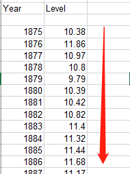
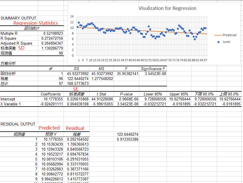
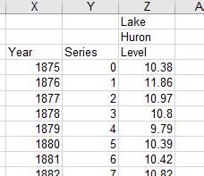
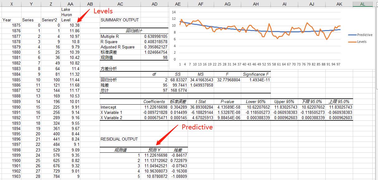
Step 1: View the original data set

Original

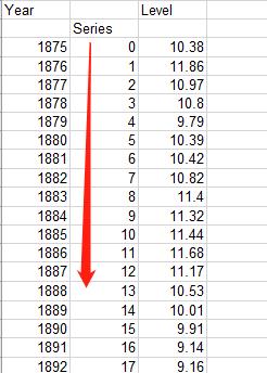
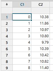
Step 2: Year subtract 1875 for starting from 0

Add New Column

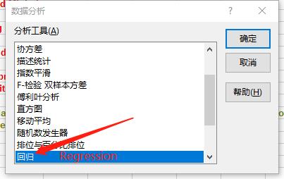
Step 3: Select Analysis tool

Analysis tool

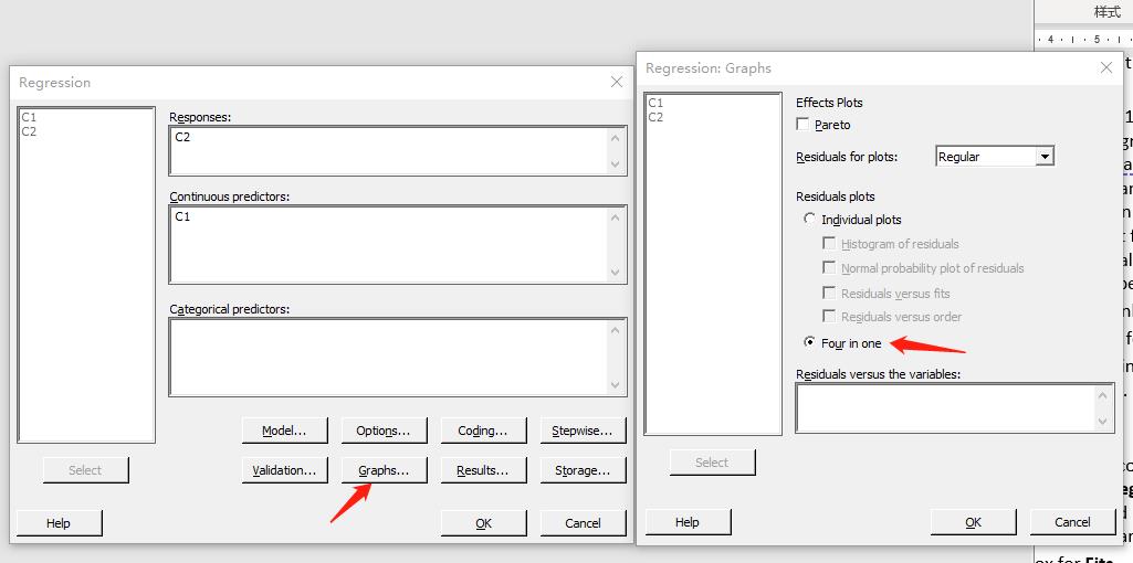
Step 4: Select regression tools

Select Regression

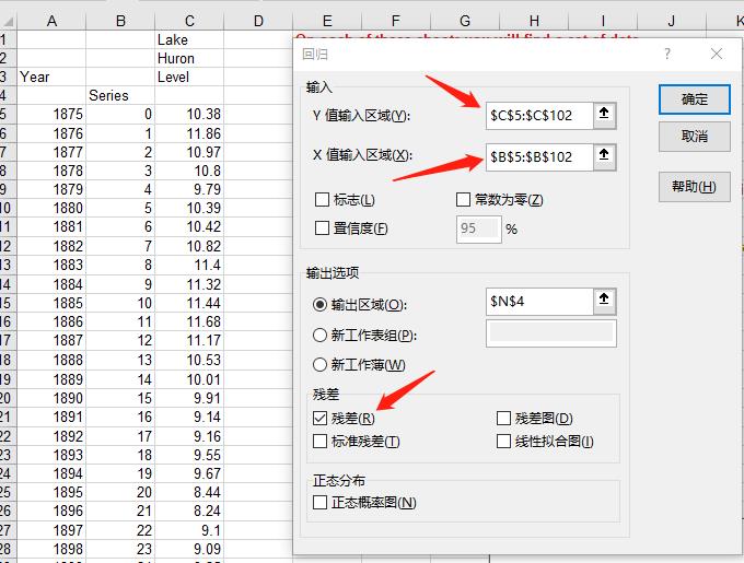
Step 5: Setting parameter for regression

Setting Parameters

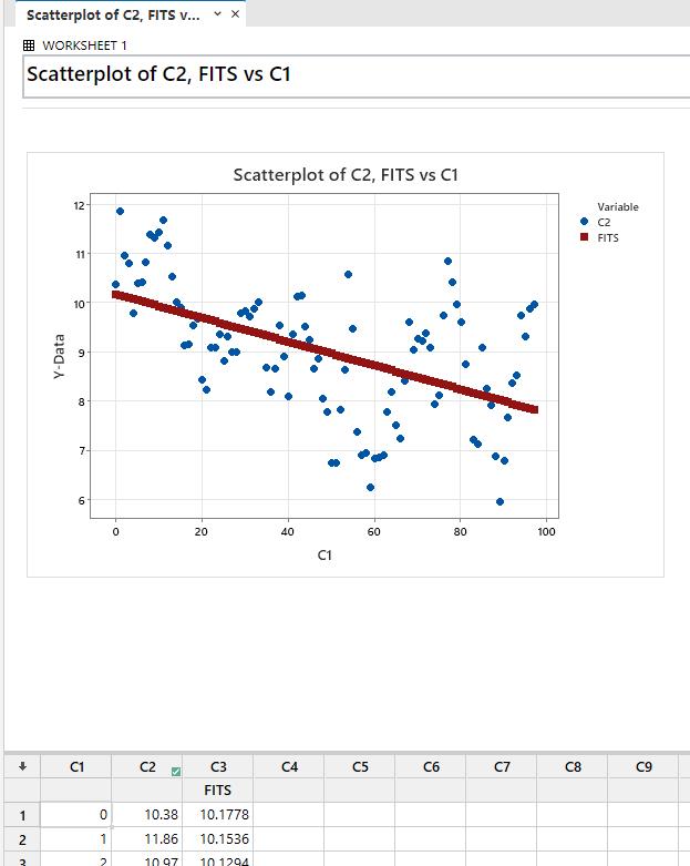
Step 6: Results and Visualization

Results

More Details of the Parameters

Please refer here for more information of each parameters

Part2: Multiple Linear Regression

Click for Steps of Multiple Linear Regression

Do Regression on $x$ and $x^2$.

Step 1: Copy Data to a New Place

Copy data

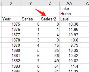
Step 2: Create new column

New column $x^2$

Step 3: Select Analysis tool and set parameters

Select tool please refer to Step3 and Step 4 from Part1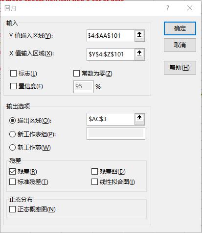

Step 4: Results

Results

Minitab: Simple Linear Regression

Download Minitab

Click for Steps on Minitab

Step 1: Copy Data to Minitab

Copy data

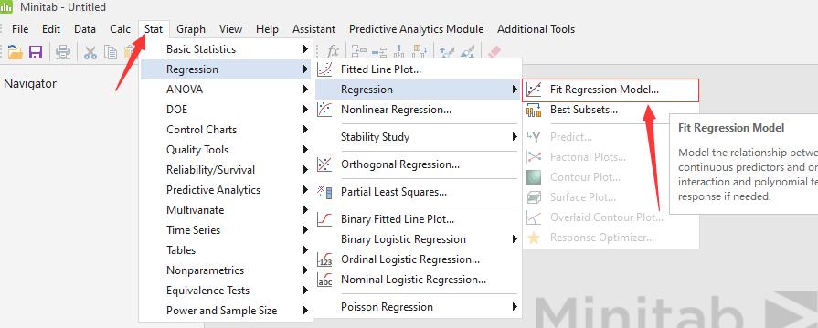
Step 2: Select Regression Tool

Tool

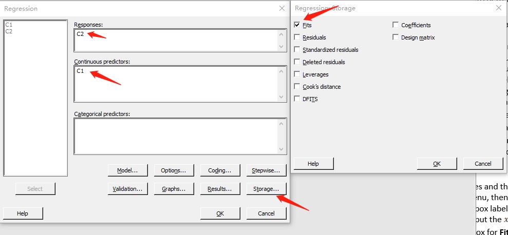
Step 3: Set Parameters

Step 4: Results

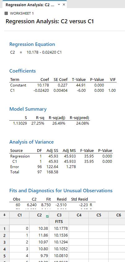
Numerical Results

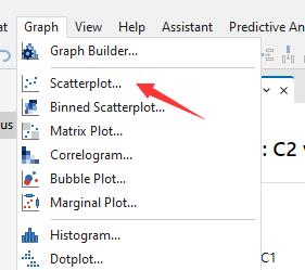
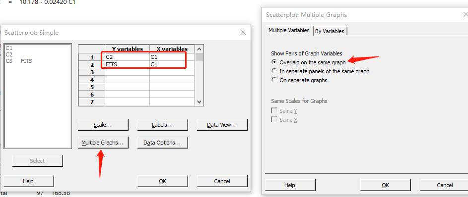
Step 5: Visualization

Select Menu

Setting Parameters

Visualization Result

Seasonality

instructions

Details

1. Make sure that you have completed Practical 1 before anything else.

2. Deaths
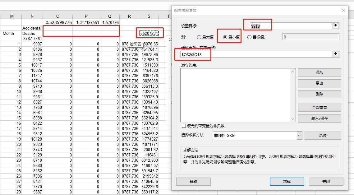
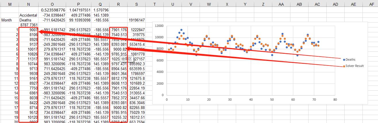
   Open the file Power_Spectrum.xls. Take your detrended series from the deaths data set, and copy it into the file starting at cell A11. Then hit the button labelled Power Spectrum. You will be asked the number of data values and how many frequencies you want.

   Then, copy columns A-B to columns M-N. In N4 put the formula =AVERAGE(N5:N76) – the mean death number. In O1 put =2*pi()/12, the frequency of one cycle per year, followed by =4*pi()/12 and =6*pi()/12 in P1 and Q1. We are about to see what cycles contribute to the seasonality. In O5 put the formula =O$2*COS(O$1*$M5)+O$3*SIN(O$1*$M5) – this will be the contribution at time t= 1 month with this frequency as soon as we estimate the coefficients that are in O2 and O3. Copy this formula across to Q5 – check how it changes. In R5 put =SUM(O5:Q5)+$N$4 – the sum of the contributions at this time from all frequencies plus the mean. In S5 we put =(N5-R5)^2 – the squared deviation of the model from the observed value. Highlight O5-S5 and copy down to row 76. In S78 put =SUM(S5:S77) – the sum of the squared deviations of the model from the observations. We want to estimate the coefficients O2-Q3 to miminise this. Go to the Data menu and select Solver. Then make selections to minimise S78 by changing cells O2:Q3. Then plot columns N and R versus M. How well does it fit? Now try the regression version I did in class – same results? What extra information do we get?

3. We are going to examine the seasonality of the red wine data now. But, this is after you have removed the trend. Open the file Power_Spectrum.xls. Take your detrended series from the red wine data set, and copy it into the file starting at cell A11. Then hit the button labelled Power Spectrum. You will be asked to input the number of data values – 132, and then the number of frequencies you want to graph – 50. Now inspect the graph and decide which frequencies you will have to include in your Fourier Series model. Then use a similar structure to that for the Deaths data set to evaluate the Fourier model. Graph the model and data together. If you are feeling adventurous, graph the original data and the combination of trend and seasonality together.

4. Repeat what you have done in Questions 2,3 for the Jeans data set.

5. Now decide how you want to fit seasonal models, using either or both of the other two approaches and try them in Matlab, r or Python.

Practice 2:: Solver

Use Solver to find an optimal (maximum or minimum) value for a formula in one cell — called the objective cell — subject to constraints, or limits, on the values of other formula cells on a worksheet. Solver works with a group of cells, called decision variables or simply variable cells that are used in computing the formulas in the objective and constraint cells. Solver adjusts the values in the decision variable cells to satisfy the limits on constraint cells and produce the result you want for the objective cell.

Put simply, you can use Solver to determine the maximum or minimum value of one cell by changing other cells. For example, you can change the amount of your projected advertising budget and see the effect on your projected profit amount.

Click for Steps for using solver

Step 1: Planning

Fill each cell using the formula below

N4 =AVERAGE(N5:N76)
 
O1 =2*PI()/12
P1 =4*PI()/12
Q1 =6*PI()/12
 
O5 =O$2*COS(O$1*$M5)+O$3*SIN(O$1*$M5)
P5 =P$2*COS(P$1*$M5)+P$3*SIN(P$1*$M5)
Q5 =Q$2*COS(Q$1*$M5)+Q$3*SIN(Q$1*$M5)
R5 =SUM(O5:Q5)+$N$4
S5 =(N5-R5)^2

S3 =SUM(S5:S77)

Drag the formulas on row 5 to fill the rest of cells.

The number after filling the formula

Step 2: Select the solver

Setting parameters 1

Step 2: Setting the parameters of solver

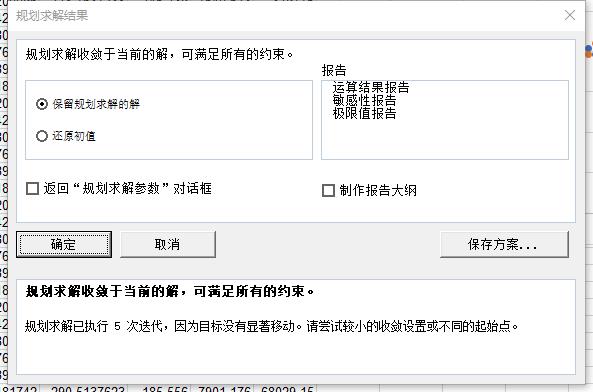
Step 2: View the result

Visualization Result

Practice 3: Prediction

Resources

Practice Week 5 (Video)

Practical video for week 5

References

1. The practice instruction from John in SP52023.
2. Software office website