05. Time series analysis (W5)

Haiyue3/23/24About 4 min

Codes on Google Collab

Predictive Analytics - Introduction: Time series analysis

Question to answer

Will a person buy a house? – Yes or no.
How much will he pay for a house? – Amount of dollars.
When will he buy a house? – A date.
How long will he keep looking for a house? – Length of time period.

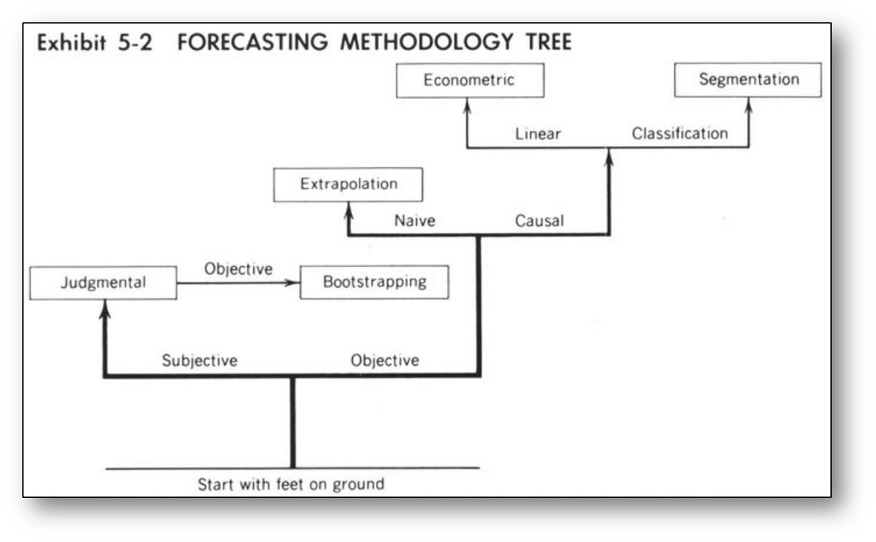
Types of Predictive analytics

Objective methods:
- Causal models
- Time series
- Artificial Intelligence (AI)
Subjective methods:
- Composites
- Surveys
- Jury of executive opinions
- The Delphi method
- Prediction or information markets
Combined Methods

Subjective forecasting

Qualitative methods
Also called: implicit, informal, clinical, experienced-based, intuitive methods, guesstimates, WAGs (wild-assed guesses), or gut feelings.
Aggregation of expert opinions:
- Sales Force Composites – aggregation of sales personnel estimates
- Jury of executive opinions
- Surveys – customer surveys, political elections polls

The Delphi Method

Interactive forecasting method which relies on a panel of experts
The Delphi method is based on the assumption that group judgments are more valid than individual judgments
Key characteristics:
- anonymity of participants;
- structuring of information flow;
- regular feedback;
- role of the facilitator.

Combined methods

Increase a number of experts
Take implicit subjective method and make it explicit and operational
Right down rules used by experts to make their decisions and then use bootstrapping to create a huge number of opinions and converge to some decision

Objective forecasting

Based on abundance of data and objective (statistical) methods of data analysis

Causal models: regression and classification models
Time series analysis: trend, seasonality, moving averages, smoothing, …
Artificial Intelligence (AI): Neural networks, Machine Learning, Deep Learning

Business questions:

What would be sales next month?
Will the client renew subscription?
Should the customer be given a home loan?
What is a probability of a customer to default?
What is weather forecast for tomorrow, next week, next season?
Causal models:
- $y = α + β_{1} x_{1} + β_{2} x_{2} + . . . + β_{n} x_{n} + ϵ$
- $y = f (x_{1}, x_{2}, . . ., x_{n})$
Time series analysis:
- $y_{t} = α + β_{1} y_{t - 1} + β_{2} y_{t - 2} + . . . + β_{n} y_{t - n} + ϵ_{t}$
- $y_{t} = f (y_{t - 1}, y_{t - 2}, . . ., y_{t - n})$
Artificial Intelligence (AI)

Forcasting Methodology Tree
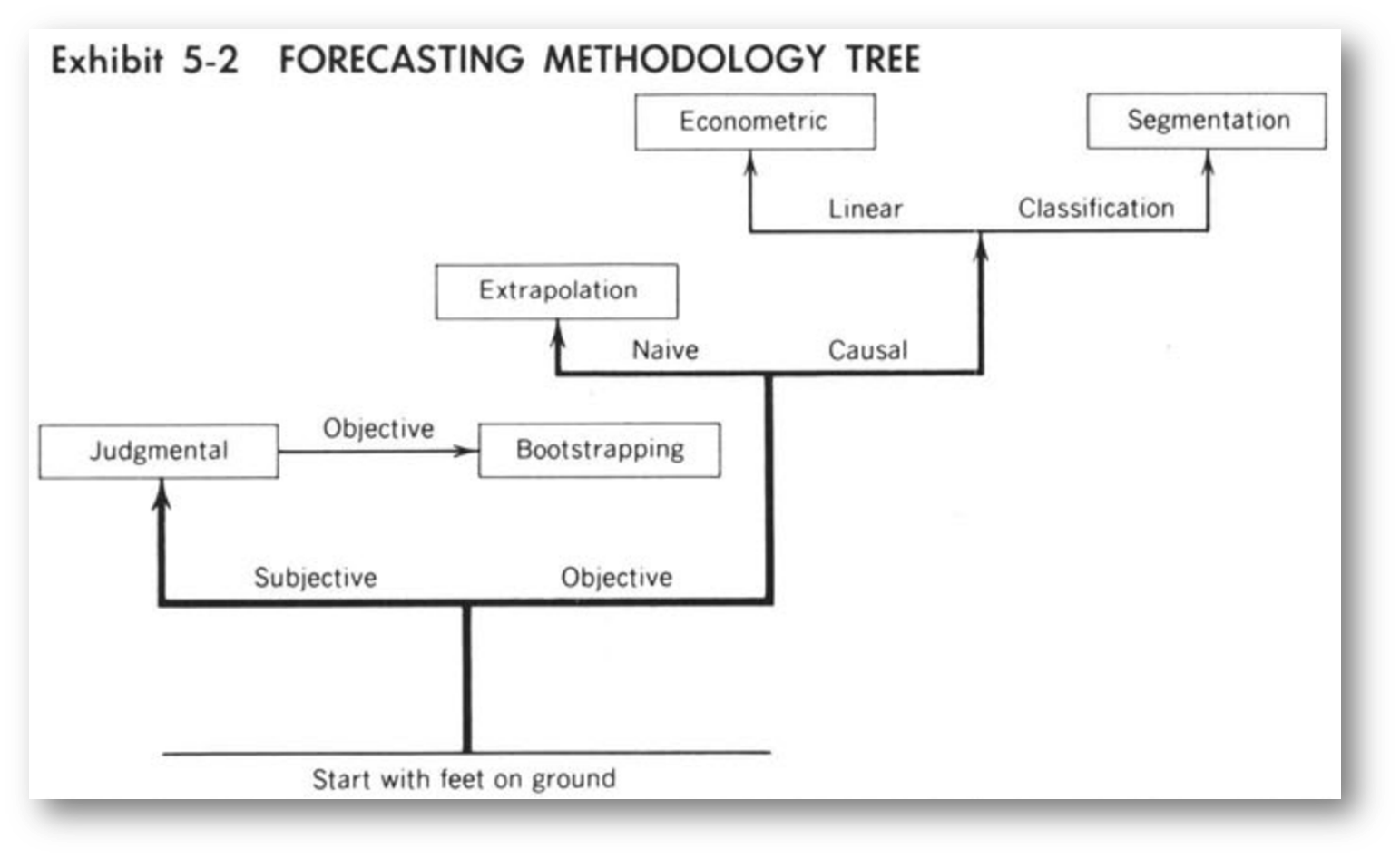
(ARMSTRONC, J. S. (1985). Long-Range Forecasting: From Cristal Ball to Computer (2nd Edn). New York: Wiley-Interscience. )

Time series

Trend

Seasonality

resource

invisible(lapply(c("readr", "dplyr", "ggplot2", "tseries"), library, character.only = TRUE))
diet <- read_csv("Diet.csv")
diet <- diet %>% mutate(Date = as.Date(Week, format="%d-%m-%y"), Type="Real") %>% select(-Week)
ggplot(data=diet, aes(x=Date, y=Diet)) + geom_line(size=1)

fit <- arima(diet$Diet[1:204], c(0, 1, 1), seasonal = list(order = c(0, 1, 1), period = 52))
pred <- predict(fit, n.ahead = 57)
diet2 <- rbind(diet, data.frame(Date=diet$Date[205:261], Diet=pred$pred, Type="Pred"))
ggplot(data=diet2, aes(x=Date, y=Diet, group=Type)) + geom_line(aes(color=Type), size=1) + theme(legend.position = c(0.1, 0.8))

(Residuals)Moving average

$M A (n)_{i} = \frac{1}{n} \sum_{j = i - n}^{i} y_{j}$

Stock Market

invisible(lapply(c("readr", "dplyr", "ggplot2"), 
            library, character.only = TRUE))
spx <- read_csv("SP 500 Historical Data.csv")
spx$Date <- as.Date(spx$Date, format="%b %d, %Y")
head(spx)
ggplot(data=spx, aes(x=Date, y=Price)) + 
        geom_line(size=1) + 
        scale_x_date(date_breaks = "1 year", 
                     date_labels =  "%Y")

spx2 <- as.matrix(spx[, c("Open","High","Low","Price")])
rownames(spx2) <- as.character(spx$Date)

library(dygraphs)
dygraph(head(spx2, 50)) %>% dyCandlestick()
head(spx2)

Random Walk

x <- data.frame(
    Date=seq.Date(as.Date("2015/1/1"),
    as.Date("2019/1/1"), by = "day")
)
x$Change <- rnorm(nrow(x), mean=0.0, sd=0.02)
x$Price <- cumprod(x$Change + 1) * 15

ggplot(data=x, aes(x=Date, y=Price)) + 
    geom_line(size=1) + 
    scale_x_date(date_breaks = "1 year", date_labels =  "%Y")
head(x)

Gambler's ruin problem

Gambler starts with some money
‘Fair game’ with 50:50 chance
Result of each game is up or down $1
For how long will the player play?
How much money will he get?

money <- 10
cnt <- 1
while(money[cnt] > 0){
  new_game <- sample(c(-1,1), size=1,
                     prob=c(0.5, 0.5))
  money <- c(money, money[cnt] + new_game)
  cnt <- cnt + 1
}
print(cnt)

Example 1

library(doSNOW); library(foreach)
cl <- makeCluster(6, type="SOCK"); registerDoSNOW(cl)
res <- foreach(i=seq(1,1000), .combine=c) %dopar% {
  money <- 10; cnt <- 1
  while(money > 0){
    new_game <- sample(c(-1,1), size=1, prob=c(0.5, 0.5))
    money <- money + new_game
    cnt <- cnt + 1
    if(cnt > 1000){
      break
    }
  }
  cnt
}

hist(res[res < 1000], breaks=50)

Example 2

library(doSNOW); library(foreach)
cl <- makeCluster(6, type="SOCK"); registerDoSNOW(cl)
res <- foreach(i=seq(1,1000), .combine=c) %dopar% {
  money <- 10; cnt <- 1
  while(money > 0){
    new_game <- sample(c(-1,1), size=1, prob=c(19/37, 18/37))
    money <- money + new_game
    cnt <- cnt + 1
    if(cnt > 1000){
      break
    }
  }
  cnt
}
hist(res[res < 1000], breaks=50)

An expected duration of the game: $D_{z} = \frac{z}{q - p}$ , where $z$ is initial capital, $𝑝$ is probability of win, $𝑞$ is probability of loss
$D_{10} = \frac{10}{19 / 36 - 18 / 36} = 360$

Trading strategies

library(readr)
library(tidyquant)
bank <- read_csv("CBA.AX.csv")

ggplot(data=bank, aes(x=Date, y=Close)) + 
  geom_line(size=0.5) + theme_bw() + 
  ggtitle("CBA stock price") +
  geom_ma(ma_fun=SMA, n=50, color="red", size=1) +
  geom_ma(ma_fun=SMA, n=200, color="blue", size=1)

Finance engineering - synthetic asset

library(readr); library(tidyquant)
CBA <- read_csv("CBA.AX.csv")
WBC <- read_csv("WBC.AX.csv")

pair <- data.frame(Date=CBA$Date, 
           Return=log(CBA$Close) - log(WBC$Close))

ggplot(data=pair, aes(x=Date, y=Return)) + 
  geom_line(size=0.5) + theme_bw() +
  ggtitle("Pair CBA-WBC")

Time series filtering

library(readr); library(dplyr)
CBA <- read_csv("CBA.AX.csv")
renko <- function(pr, H){
  res <- data.frame(Time=1, Return=pr[1])
  for(i in seq(2, length(pr))){
    if(abs(pr[tail(res$Time,1)] - pr[i]) >= H){
      res <- res %>% add_row(Time=i, Return=pr[i])
    }
  }
  return(res)
}

ren <- renko(log(CBA$Close), H=0.1)
ren$Date <- CBA$Date[ren$Time]

ggplot(data=CBA, aes(x=Date, y=log(Close))) + geom_line(size=0.5, col="#00BFC4") + theme_bw() + ggtitle("CBA returns") + geom_line(data=ren, aes(x=Date, y=Return), size=1, col="#F8766D") + geom_point(data=ren, aes(x=Date, y=Return), size=2, col="#F8766D")

Stock market

First parameters
- $ξ = 1.75$
- $H = 0.05$
Second parameters
- $ξ = 1.92$
- $H = 0.01$
Third parameters
- $ξ = 1.41$
- $H = 0.05$

get_xi <- function(pr){
  temp <- sign(diff(pr))
  temp <- sapply(seq(2, length(temp)),
          function(i) temp[i-1] != temp[i])
  return(1 / mean(temp))
}
get_xi(ren$Return)

Summary

Predictive analytics: subjective and objective
Subjective forecasting:
- Aggregation of expert opinions, Delphi method, Information markets
Objective forecasting: naive and causal
- Time series - naive forecasting
- Random Walk - impossible to make predictions
- Time series transformation and filtering

Don’t Gamble! …unless you understand the process in details and probability is on your side.

Reference

Tim's slides of Week 5