02. Descriptive Analytics (W2)

A/B testing and Discrete Choice Experiments

Playing golf

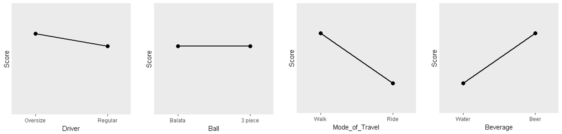
What influences a score?

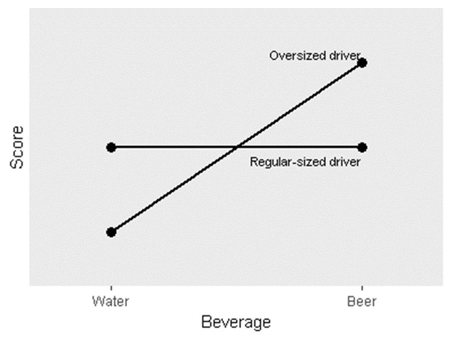
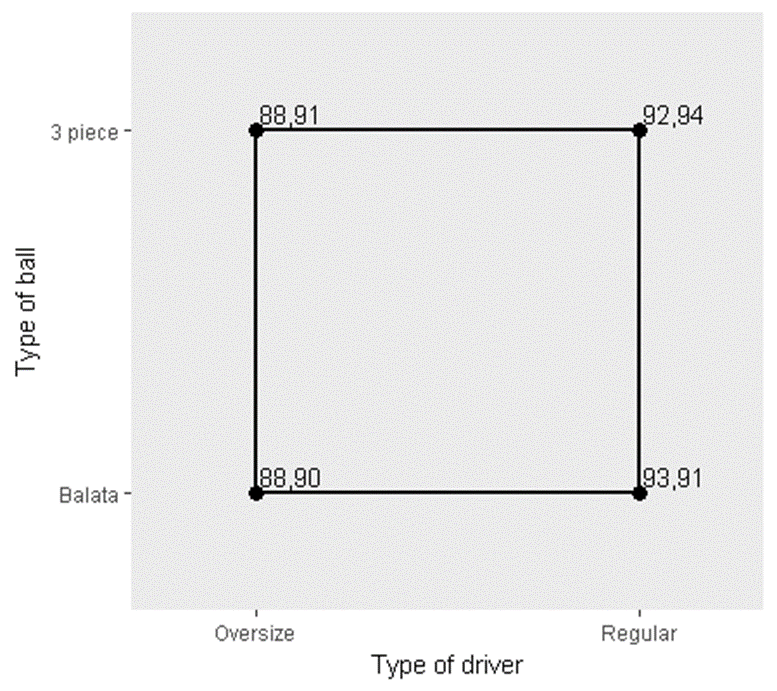
• The type of driver used (oversized or regular size)
• The type of ball used (balata or three pieces)
• Walking and carrying the golf clubs or riding in a golf cart
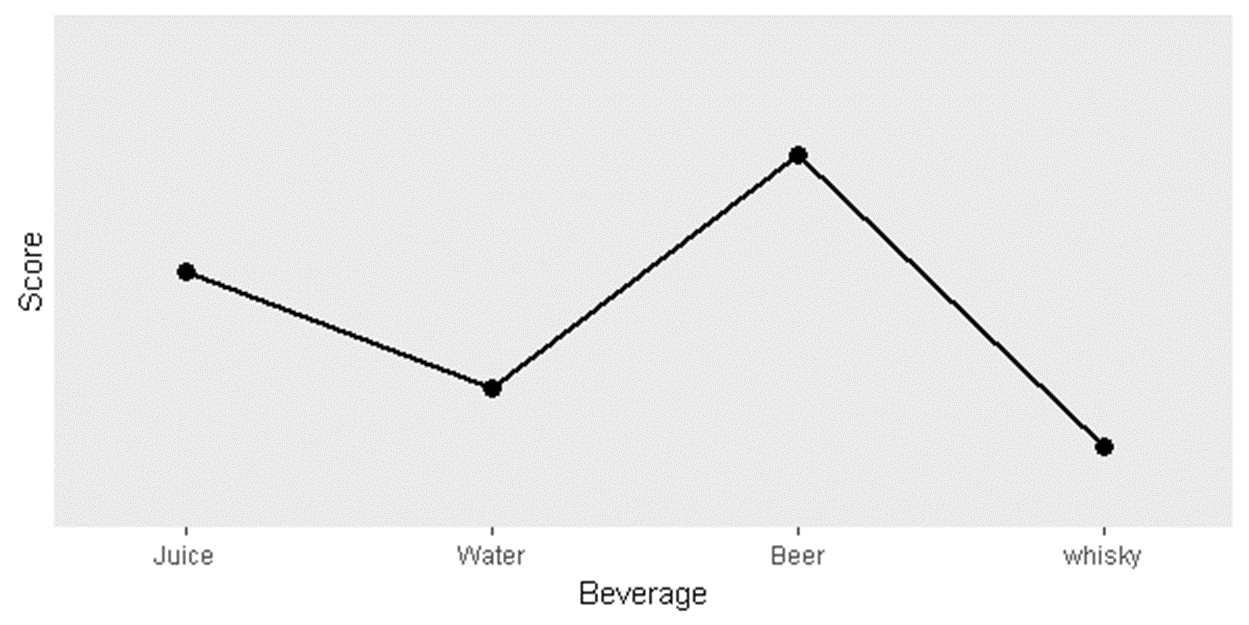
• Drinking water or drinking beer while playing
• Playing in the morning or playing in the afternoon
• Playing when it is cool or playing when it is hot
• The type of golf shoe spike worn (metal or soft)
• Playing on a windy day or playing on a calm day

One-factor-at-a-time strategy

T-Test

ANOVA

$2^2$ factorial design

Interaction between type of driver and type of beverage for golf experiment

type of driver

$Divereffect=\frac{92+94+93+91}{4}-\frac{88+91+88+90}{4}=3.25$
$Balleffect=\frac{92+94+93+91}{4}-\frac{88+91+88+90}{4}=0.75$
$Drive-Ballinteractioneffect=\frac{88+90+92+94}{4}-\frac{88+91+93+91}{4}=0.25$

Discrete (Stated) Choice Experiment

3 factors

• HACCP label: (Yes/No)
• Eco label: (Yes/No)
• Price: (145, 150, 155, or 160 yen)

Aizaki, H. and Nishimura, K., 2008. Design and analysis of choice experiments using R: a brief introduction. Agricultural Information Research, 17(2), pp.86-94.

Full Factorial Design

library(AlgDesign)
ffd <- gen.factorial(
    c(2,2,4),
    varNames = c("HAC", "ECO", "PRI"),
    factors="all"
)
ffd

	HAC	ECO	PRI
1	1	1	1
2	2	1	1
3	1	2	1
4	2	2	1
5	1	1	2
6	2	1	2
7	1	2	2
8	2	2	2
9	1	1	3
10	2	1	3
11	1	2	3
12	2	2	3
13	1	1	4
14	2	1	4
15	1	2	4
16	2	2	4

Discrete Choice Experiment

Consider a product with the following three attributes:

• The region of origin: Region A, Region B, Region C
• The eco-friendly label:
  • “Conv.” (conventional cultivation method),
  • “More” (more eco-friendly cultivation method), and
  • “Most” (most eco-friendly cultivation method)
• The price per piece of the product: $1, $1.1, $1.2

Design

library(support.CEs)
des1 <- rotation.design(
    attribute.names = list(
        Region = c("Reg_A", "Reg_B", "Reg_C"),
        Eco = c("Conv.", "More", "Most"),
        Price = c("1", "1.1", "1.2")),
    nalternatives = 2, 
    nblocks = 1, 
    row.renames = FALSE,
    randomize = TRUE, 
    seed = 987
)

questionnaire(choice.experiment.design = des1)

Collected data

## https://cran.r-project.org/web/packages/support.CEs/support.CEs.pdf
data("syn.res1")
syn.res1[1:3, ]

desmat1 <- make.design.matrix(
    choice.experiment.design = des1,
    optout = TRUE, 
    categorical.attributes = c("Region", "Eco"),
    continuous.attributes = c("Price"), 
    unlabeled = TRUE
)
desmat1[1:3, ]

dataset1 <- make.dataset(
    respondent.dataset = syn.res1,
    choice.indicators = c("q1", "q2", "q3", "q4", "q5", "q6", "q7", "q8", "q9"),
    design.matrix = desmat1
)
dataset1[1:10, ]

Analysis - clogit

library(survival)
clogout1 <- clogit(
    RES ~ ASC + Reg_B + Reg_C + More + Most + Price + strata(STR), 
    data = dataset1
)
clogout1 <- clogit(
    RES ~ ASC + Reg_B + Reg_C + More + Most + More:F + Most:F + Price + strata(STR), 
    data = dataset1
)
clogout1

• tips

  Info

  Results interpretation is the same as in “normal” Logistic Regression Analysis.

Analysis - Goodness of Fit

gofm(clogout1)

Analysis – MWTP

Marginal Willingness to Pay (MWTP)

mwtp(
    output = clogout1, 
    monetary.variables = c("Price"), 
    nonmonetary.variables = c("Reg_B", "Reg_C", "More", "Most", "More:F", "Most:F"),
    confidence.level = 0.90,
    seed = 987
)

Summary

• Causal research as a part of Descriptive Analytics
• Experiment design
• A/B testing
• Discrete choice experiments
  • Full and partial factorial design
  • Design, data collection, analysis, interpretation
  • Marginal willingness to pay

Reference

Tim's slides of Week 2