04. Probability distributions (W4)

Haiyue3/23/24About 5 min

Descriptive Analytics - Probability distributions
Codes on Google Collab

Predictive analytics VS randomness

What is a prediction?
Is prediction possible?
What do we predict?

Bernoulli trial

A random experiment with only two possible outcomes:
- “Success” and “Failure”
- Red and Black, Head and Tail, win or lose
- Customer renewed subscription, made a purchase, repaid a loan, or not
Probability of “success” 𝑝 is always the same

𝑝=1−𝑞,
𝑞=1−𝑝,
𝑝+𝑞=1
$𝑝 = \frac{𝑆}{(𝑆 + 𝐹)}$ ,
$𝑞 = \frac{𝐹}{(𝑆 + 𝐹)}$

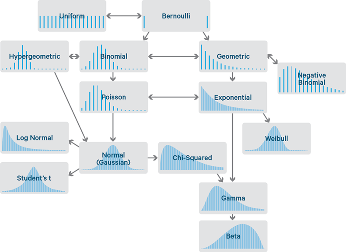
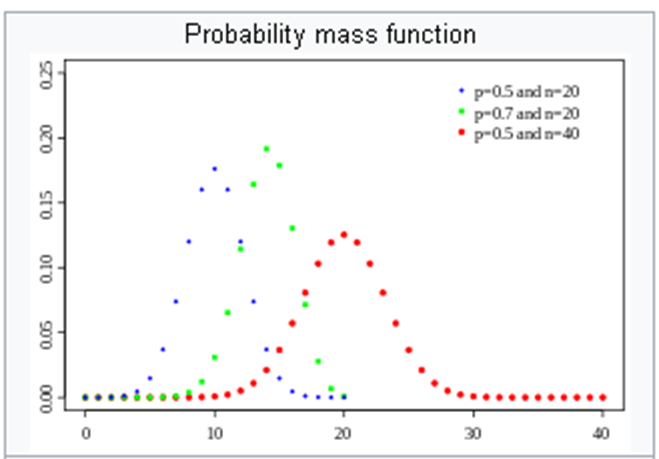
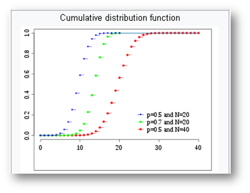
Binomial distribution

𝑛 random independent Bernoulli trials with fixed probability of “success” 𝑝
Let 𝑋 be the number of successes after 𝑛 trials
$𝑃 (𝑋 = 𝑟) = (\binom{n}{r}) 𝑝^{𝑟} (1 - 𝑝)^{(𝑛 - 𝑟)}$
Where $(\binom{n}{r})$ is a binomial coefficient, or a number of unordered selections of 𝑟 objects out of 𝑛 objects
$(\binom{n}{r}) = \frac{𝑛!}{𝑟! (𝑛 - 𝑟)!}$
Other notations are $𝐶 (𝑛, 𝑟)$ and $𝐶_{𝑟}^{𝑛}$

Example 1

A test with 10 multiple-choice questions. Each question has three possible answers.
Let’s assume that student does not know the topic at all, then the probability to get the right answer in a question is $𝑝 = 1 ∕ 3$
What is an expected result for this student?

$μ = 𝑛 𝑝 = 10 * \frac{1}{3} = 3.33$
$σ = \sqrt{n p (1 - p)} = \sqrt{10 * \frac{1}{3} * \frac{2}{3}}$
Binomial Distribution

What is a probability this student passes the test (gets 50% or more)?

\begin{aligned} P (X \geq 5) & = P (X = 5) + P (X = 6) + P (X = 7) + . . . + P (X = 10) \\ = 1 - P (X \leq 4) \\ = 1 - \sum_{i = 0}^{4} (\binom{10}{i}) p^{i} (1 - p)^{10 - i} \\ = . . . \end{aligned}

1-sum(dbinom(seq(0, 4), 10, 1/3))

What is a probability this student passes the test with 100 questions?

\begin{aligned} P (X \geq 50) & = 1 - P (X \leq 49) \\ = 1 - \sum_{i = 0}^{49} (\binom{100}{i}) p^{i} (1 - p)^{100 - i} \\ = . . . \end{aligned}

1 - sum(dbinom(seq(0,49),100,1/3))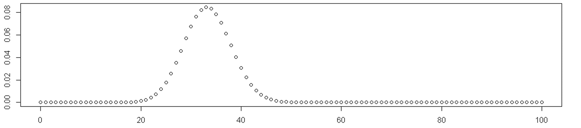

Example 2

Customers arrive to your store. You know that approximately one in four customers will buy your product, while others just shop around.
How many units will you sell if there are 100 customers per day?
$𝐸 [𝑋] = n p = 100 * 0.25 = 25$
What are upper and lower bounds for the number of units sold?

qbinom(c(0.025,0.5,0.975),100,1/4)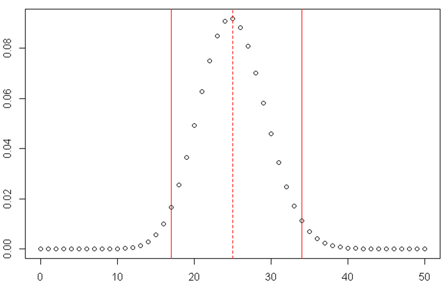

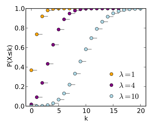
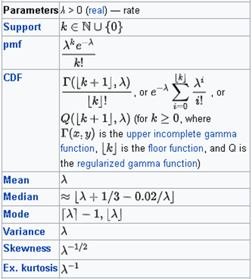
Poisson distribution

Events occur independently, at random, at a rate 𝜆 per unit time. We want to count the number 𝑋of events happening in a given time 𝑡.
$P (X = r) = \frac{e^{- λ t} (λ t)^{r}}{r!}$

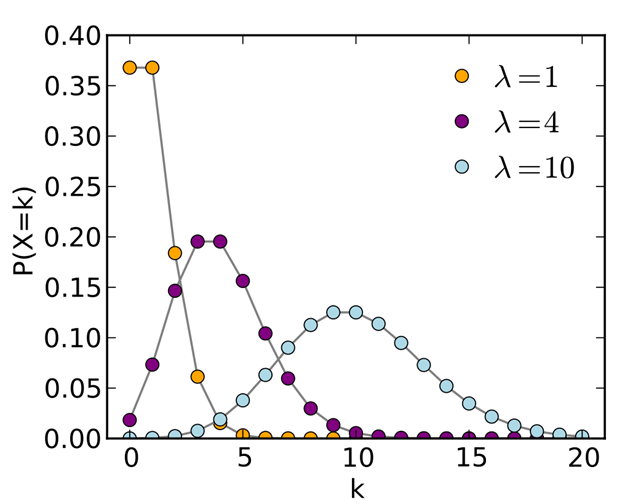
Example

There are 10 customers arriving to your store every day IN AVERAGE. What is probability that on some day there would be 15 customers or more?

\begin{aligned} P (X \geq 15) & = 1 - P (X \leq 14) \\ = 1 - e^{- 10} \sum_{i = 0}^{14} \frac{10^{i}}{i!} \end{aligned}

1-sum(dpois(seq(0, 14), lambda=10))

The Poisson distribution is often described as “the distribution of small numbers”.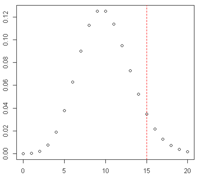
Poisson Eistribution Example

Negative Binomial Distribution

There is a sequence of independent and identically distributed Bernoulli trials with probability of success 𝑝.
We want to know the number of successes happen before 𝑟 failures.

Example:

We roll a dice and consider number “1” as failure and any other number as a success. That is, 𝑝=5∕6
How many “successes” do we get before getting three failures, that is, before we see “1” in a third time, so 𝑟=3
$P (X = k) (\binom{k + r - 1}{k}) (1 - p)^{r} p^{k}$

plot(dnbinom(seq(1,35), size=3, prob=1/6))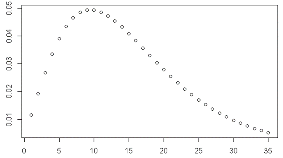

“Overdispersed Poisson”
A mixture of Poisson distributions, where rate 𝜆 is itself a random variable, distributed as a gamma distribution with shape 𝑟 and scale 𝜃=𝑝(1−𝑝)

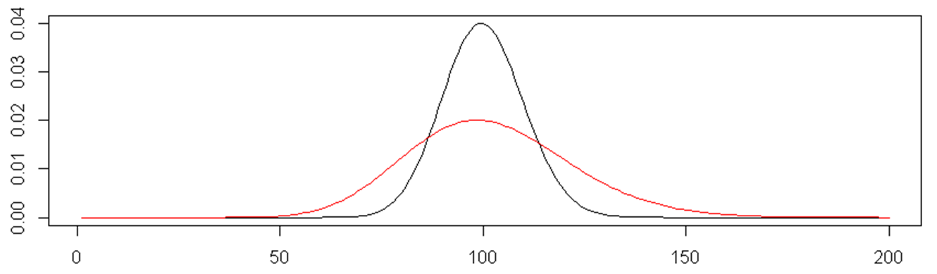
Negative Binomial Distribution Overdispersed Poisson

plot(dpois(seq(1,200), lambda=100), type="l") 
lines(dnbinom(seq(1,200), size=34, prob=0.25), col="red")

Examples

Number of job interview you have to go on before you get a job
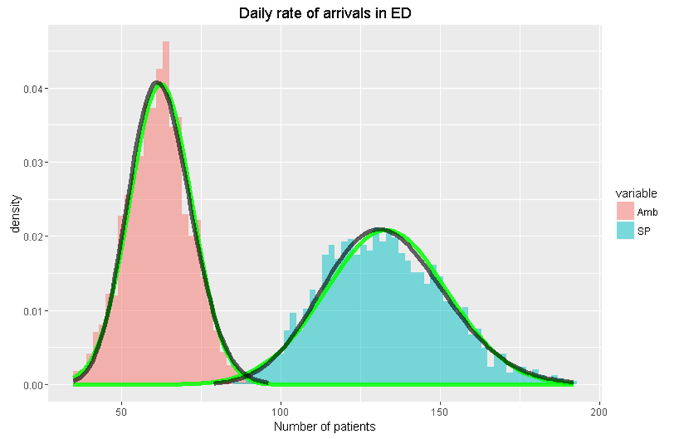
Number of patients arriving to Hospital Emergency Department
Number of customers coming to supermarket
Occurrence of tropical cyclones in North Atlantic and winter cyclones over Europe
How long an engine part will work till it gets broken and need replacement or repair

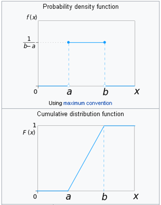
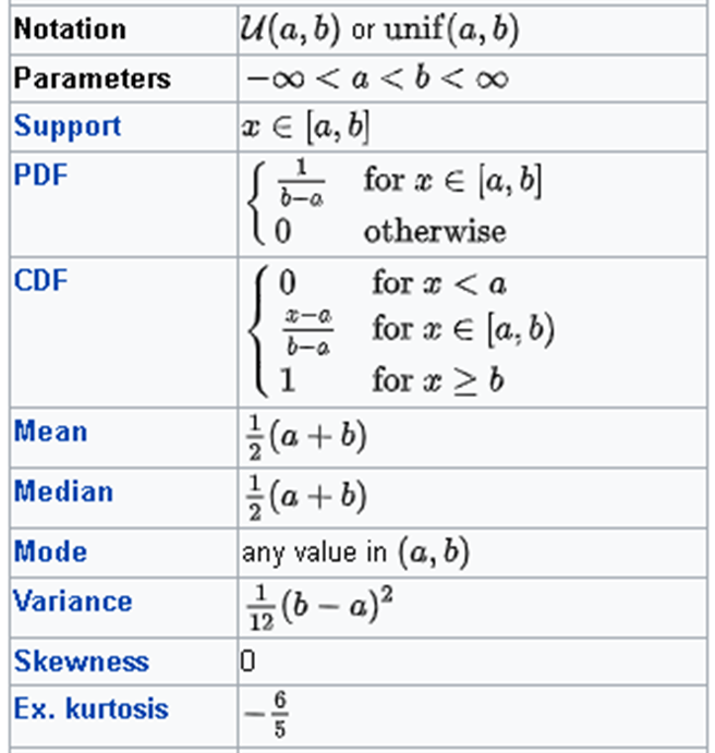
Uniform distribution

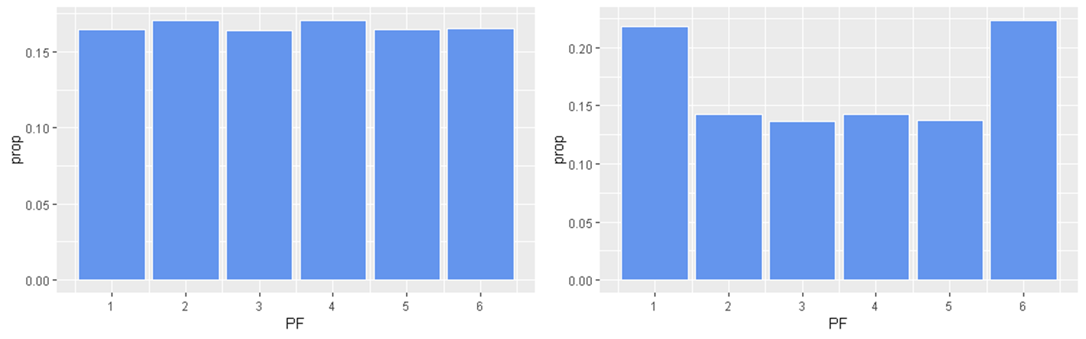
x <- sample.int(6, size=6000, replace=TRUE)
plot(table(x))
abline(h=1000, col="red", lty=2)

x <- runif(6000)
hist(x, breaks=10)
abline(h=600, col="red", lty=2)

Uniform distribution (continuous)

Very often we say that [variable] is “uniformly distributed”

if customers show no preferences towards any particular product
if there is no effect of on the variable from the selected predictors
If there is no difference between groups

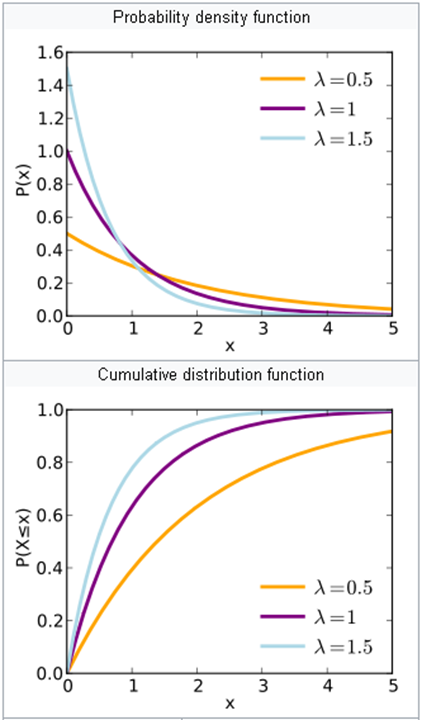
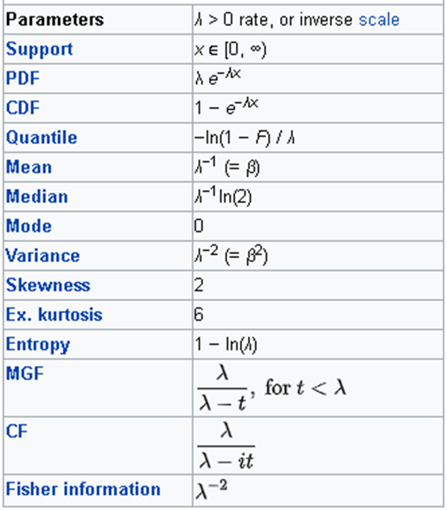
Description Uniform Distribution Continuous

Exponential distribution

If we assume that events occur according to Poisson distribution with a rate 𝜆 then waiting time 𝑇 before [next] event follows exponential distribution

\begin{aligned} F_{T} (t) & = P (T \leq t) \\ = 1 - e^{λ t} \end{aligned}

Example

Exponential distribution can be used to estimate time between different kinds of events:

Time between jobs arrivals to a service centre
Time to a component failure (lifetime of a component)
Time required to repair a component
How long to wait for the next phone call
How long to wait for a next customer to arrive

Paradox

Suppose you join a queue in a bank, with just one customer in front of you, already in service.
The time you have to wait for that customer to finish being served is independent of how long that customer has already been in service!
Exponential distribution is memoryless.
If you have been waiting time 𝑠 for the first event, what is probability that you will wait a further time 𝑡?

\begin{aligned} P (T > t + s | T > s) & = \frac{P ({T > t + s} \cap {T > s})}{P (T > s)} \\ = \frac{P (T > t + s)}{P (T > s)} \\ = \frac{e^{- λ (t + s)}}{e^{- λ s}} \\ = e^{- λ t} \end{aligned}

Hence, your remaining waiting time does not depend on time 𝑠 you already have been waiting.

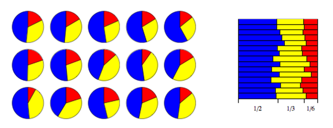
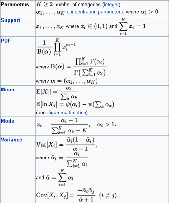
Dirichlet distribution

Market share:
Company A – 50%
Company B – 33%
Company C – 17%

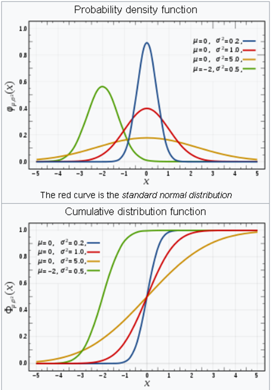
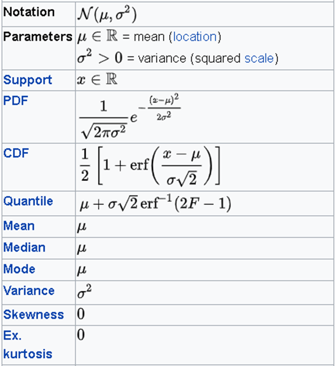
Normal Distribution

Gaussian distribution
Continuous two parameter distribution
Arises in many biological and sociological experiments
Limiting distribution in many situations

Poisson

df <- data.frame(PF = rpois(1000, lambda=50))
ggplot(df, aes(x = PF)) + 
  geom_histogram(aes(y =..density..), binwidth=2) +
  stat_function(fun = dnorm, 
  args = list(mean = mean(df$PF), sd = sd(df$PF)),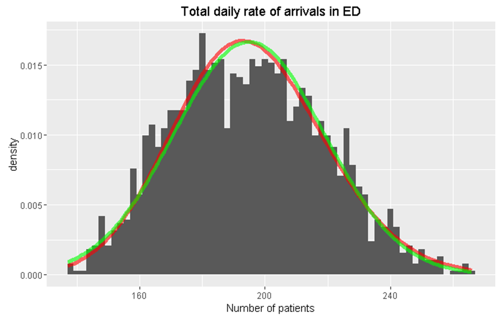
  col="red", size=2)

NBD

df <- data.frame(PF = rnbinom(1000, size=34, prob=0.25))
ggplot(df, aes(x = PF)) + 
  geom_histogram(aes(y =..density..), binwidth=5) +
  stat_function(fun = dnorm, 
                args = list(mean = mean(df$PF), 
                                   sd = sd(df$PF)),
                col="red", size=2) +
  stat_function(fun = function(x) dpois(as.integer(x), 
                lambda = mean(df$PF)) ,
                color = "green", size = 1)

Uniform

x <- matrix(runif(120000),10000,12)
df <- data.frame(PF=apply(x,1,sum)-6)
ggplot(df, aes(x = PF)) + 
  geom_histogram(aes(y =..density..), binwidth = 0.1) +
  stat_function(fun = dnorm, 
                args = list(mean = mean(df$PF), sd = sd(df$PF)),
                col="red", size=2)

Exponential

x <- matrix(rexp(120000),10000,12)
df <- data.frame(PF=apply(x,1,sum))
ggplot(df, aes(x = PF)) + 
  geom_histogram(aes(y =..density..), binwidth = 1) +
  stat_function(fun = dnorm, 
                args = list(mean = mean(df$PF), sd = sd(df$PF)),
                col="red", size=2)

Mixture distribution

$f (x) = \sum_{i = 1}^{n} w_{i} p_{i} (x)$

Non-homogenous distributions

Let’s assume that cars arrive at an intersection with some rate 𝜆 cars per hour.
Now, assume that 𝜆 is not constant but a function of time 𝜆(𝑡). That is, more cars during the day and less during the night.
Arrivals process is a non-homogenous Poisson process.
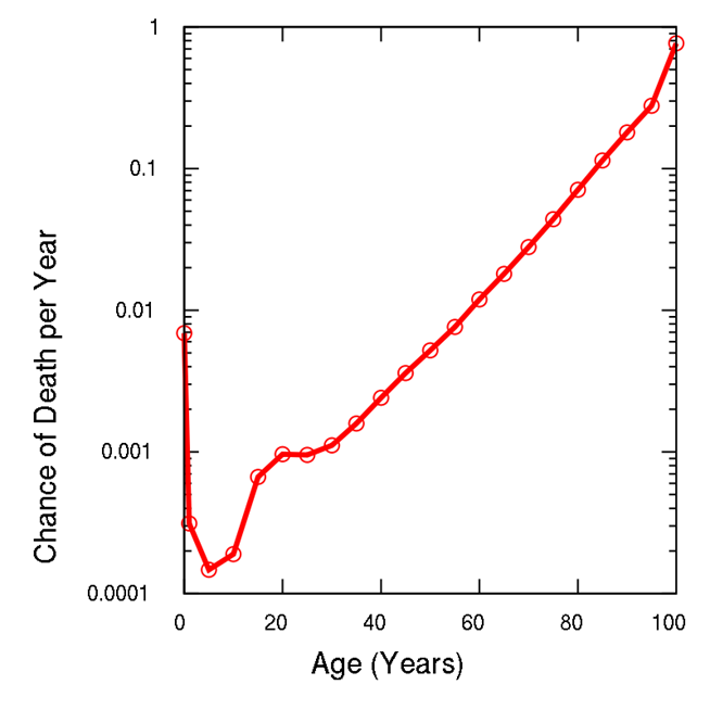
Time of arrival becomes not exponential but somewhat different, depending on the function of time 𝜆(𝑡). Often used in actuarial science, e.g. see Gompertz–Makeham law of mortality

Non-parametric distributions

Parametric distributions are distributions that can be completely described by their parameters, like 𝑁(𝜇, 𝜎^2).
Non-parametric or empirical distributions do not assume that data drawn from any known parametric distribution

Summary

Predictions about data:

central tendency,
dispersion,
most popular,
max or min values.

Reference

Tim's slides of Week 4