 Practices Part1
Week 2: Naive Bayes (Practical 1)
Part1 : Training
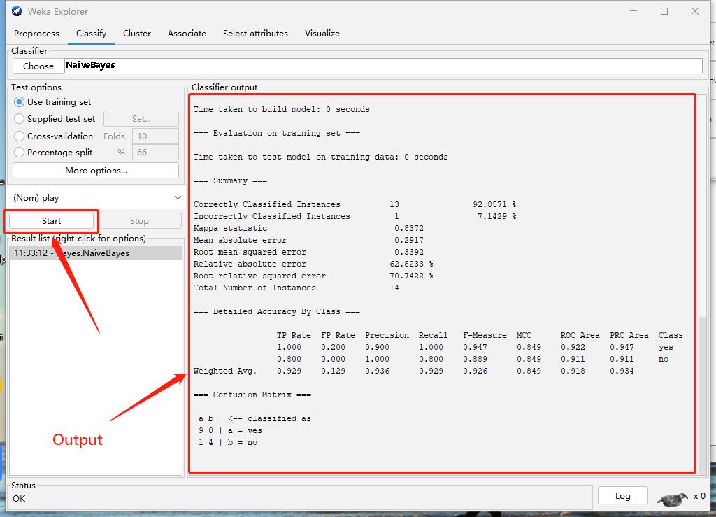
Steps of using Weka
Step1: Explorer

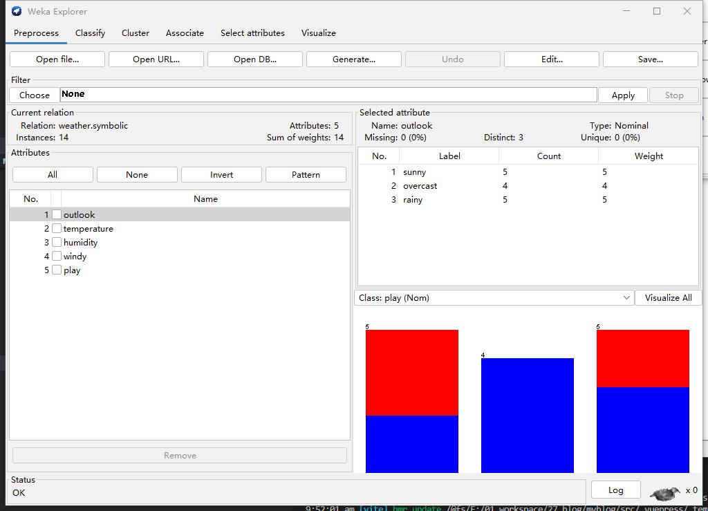
Step2: Select data

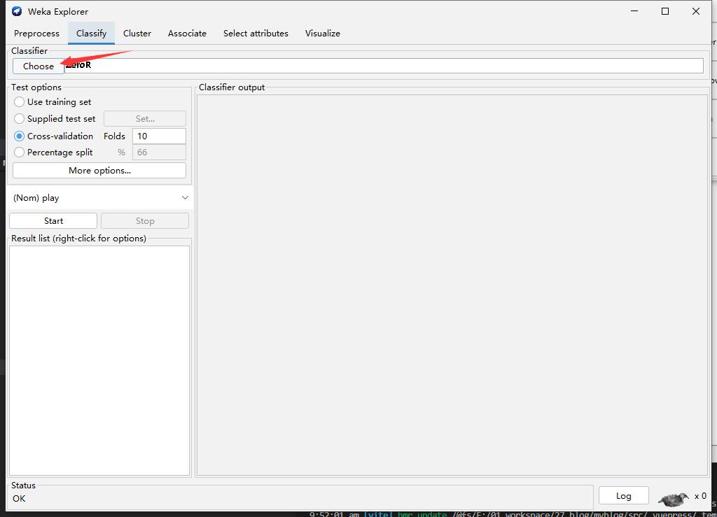
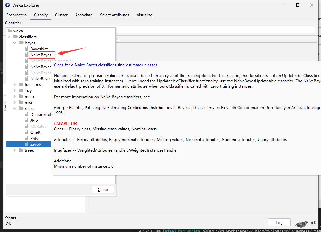
Step3: Choose Algorithm
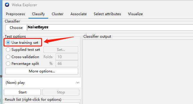
Step3: Start and Result
Part2 : Test
Test Naive Bayes Model
Step1: Create Test Data

Step2: Select Test data
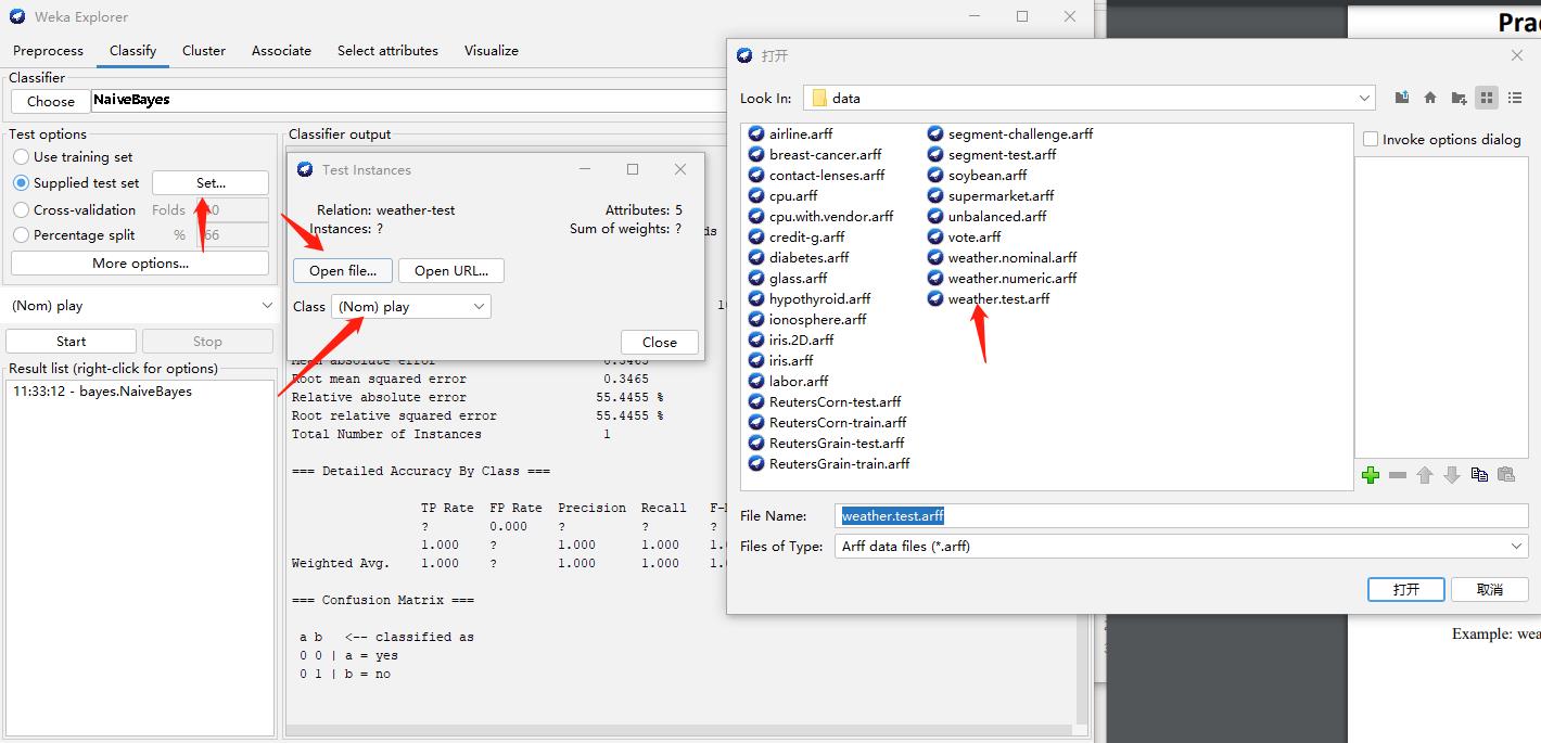
Step3: Result
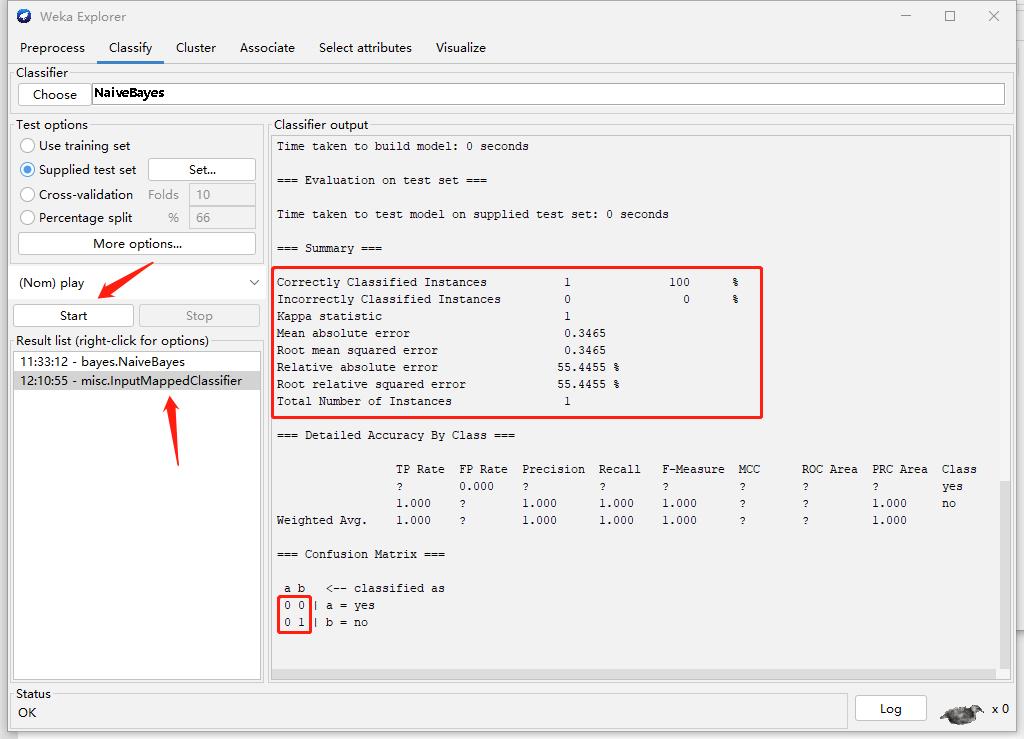
Part3 : Naive Bayes using Numerical Dataset
Steps for Numerical Dataset
Step1: Select Numerical Data
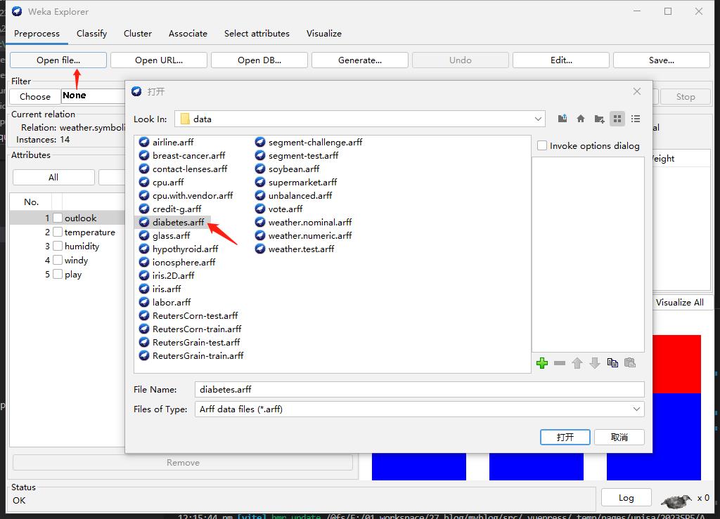
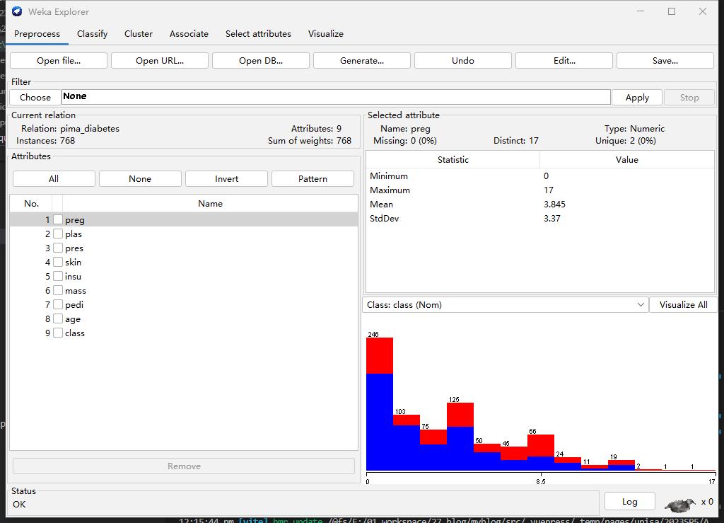
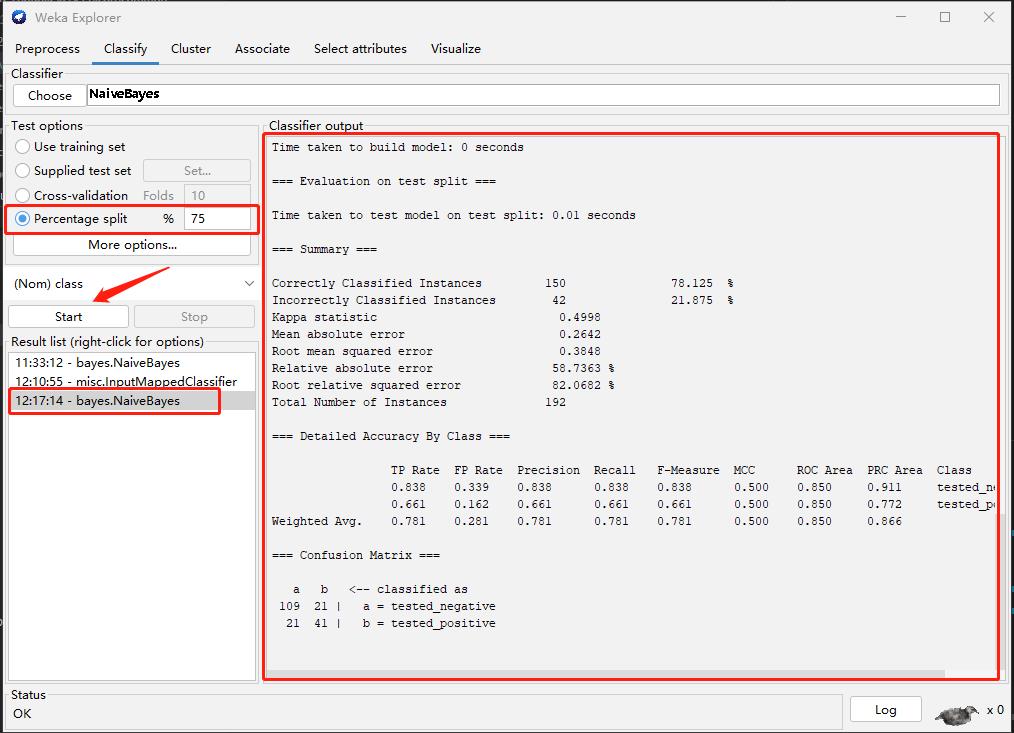
Step2: Training and Testing
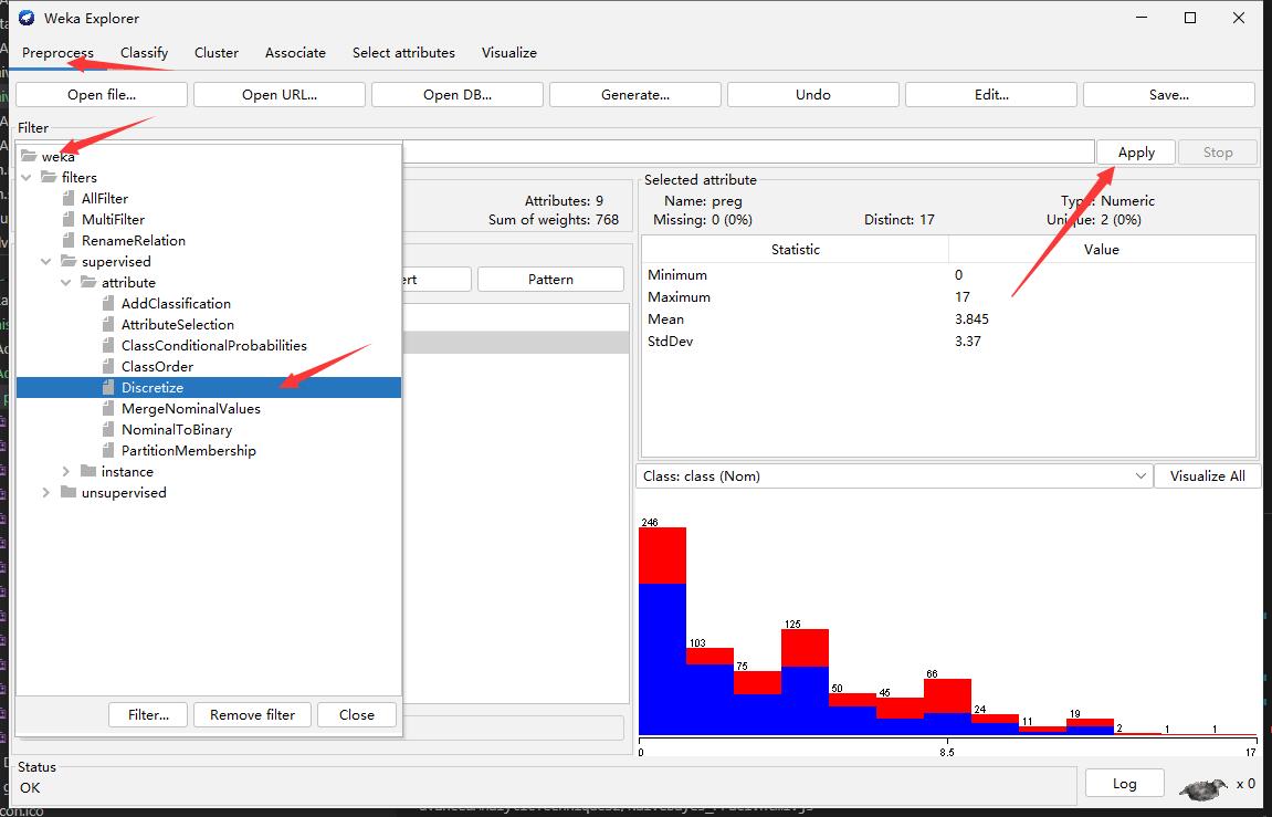
Step3: Discretize
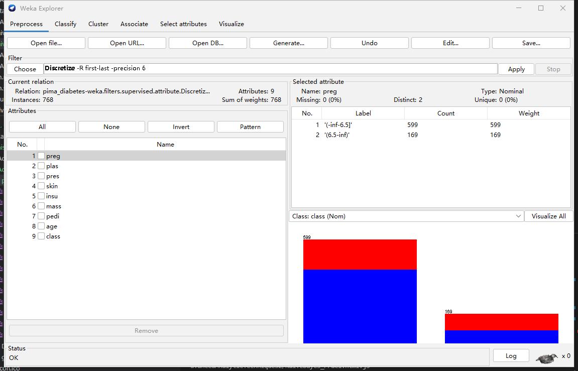
Step4: Retraing (Compare the different with Step 2)
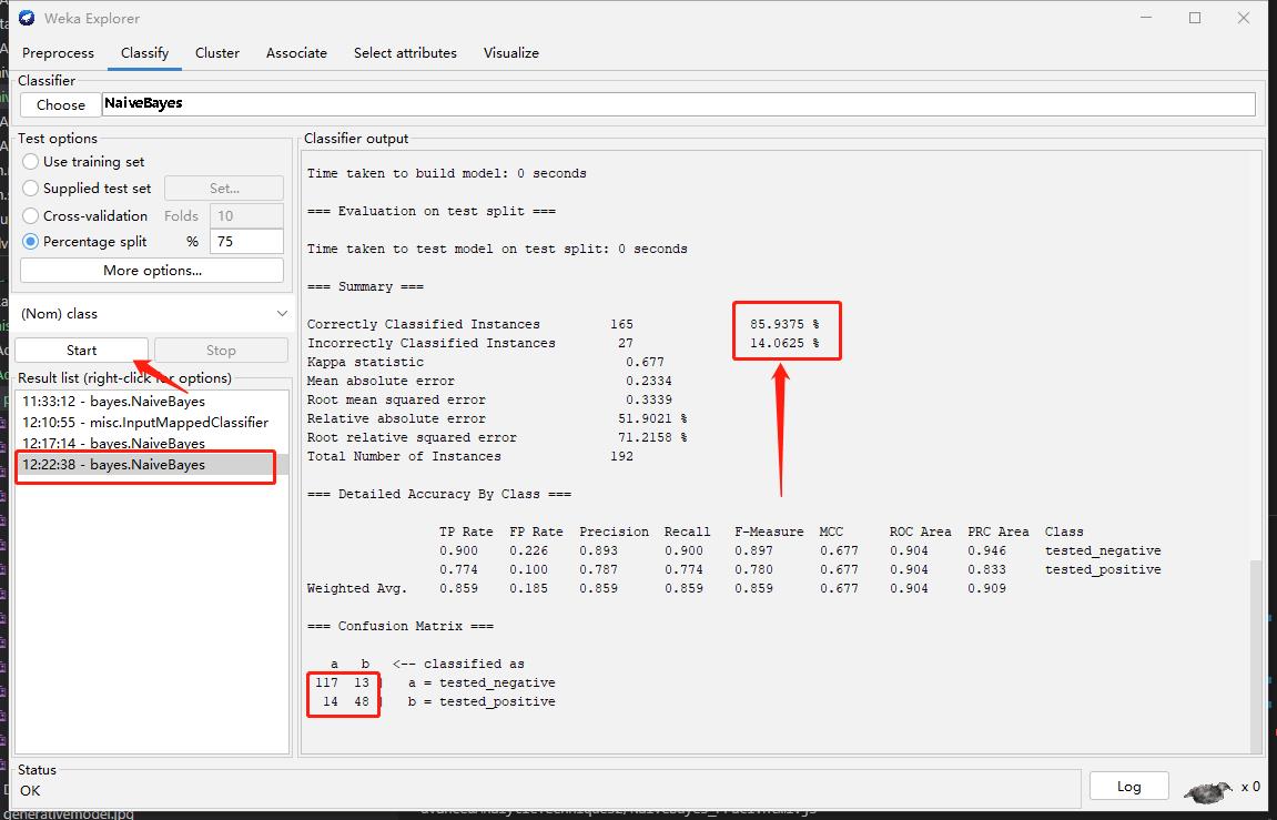
My observation
The performance increase after discretizing.
Week 3: Bayesian Network Inference (Practical 2)
Install package
if (!requireNamespace("BiocManager", quietly = TRUE))
    install.packages("BiocManager")
BiocManager::install(c("graph", "RBGL", "Rgraphviz"))

install.packages('gRain', , dependencies=TRUE)
Create the conditional probability table for the Asia network
library(gRain)

yn <- c("yes","no")

a <- cptable(~asia, values=c(1,99),levels=yn)
t.a <- cptable(~tub|asia, values=c(5,95,1,99),levels=yn)
s <- cptable(~smoke, values=c(5,5), levels=yn)
l.s <- cptable(~lung|smoke, values=c(1,9,1,99), levels=yn)
b.s <- cptable(~bronc|smoke, values=c(6,4,3,7), levels=yn)
e.lt <-
cptable(~either|lung:tub,values=c(1,0,1,0,1,0,0,1),levels=yn)
x.e <- cptable(~xray|either, values=c(98,2,5,95), levels=yn)
d.be <- cptable(~dysp|bronc:either, values=c(9,1,7,3,8,2,1,9),
levels=yn)
plist <- compileCPT(list(a, t.a, s, l.s, b.s, e.lt, x.e, d.be))
plist
#Checking the (conditional) probability of some nodes
plist$tub
plist$either
Draw the network
net1=grain(plist)
plot(net1)
Convert data into table
plist$tub %>% as.data.frame.tableQuery the marginal probabilities P(lung) and P(bronc):
querygrain(net1, nodes=c("lung","bronc"), type="marginal")Query the joint probability P(lung, bronc):
querygrain(net1, nodes=c("lung","bronc"), type="joint")Query the conditional probability P(lung|bronc)
querygrain(net1, nodes=c("lung","bronc"), type="conditional")Result
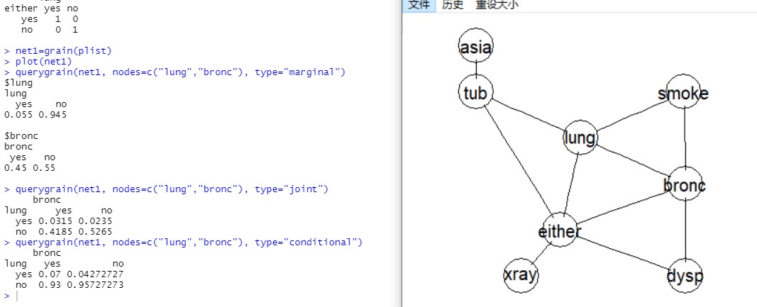
More quesitons
querygrain(net1, nodes=c("bronc"), type="marginal")
querygrain(net1, nodes=c("bronc"), type="conditional")

querygrain(net1, nodes=c("lung","bronc"), type="joint")
querygrain(net1, nodes=c("lung","smoke"), type="conditional")
querygrain(net1, nodes=c("xray","smoke"), type="conditional")
querygrain(net1, nodes=c("xray","smoke", "asia"), type="conditional")

querygrain(net1, nodes=c("lung", "asia"), type="conditional")
querygrain(net1, nodes=c("bronc", "smoke"), type="conditional")
Calculate the following probabilities:
- P(lung=yes,bronc=yes) : 0.07
- P(bronc=yes) :0.45
- P(lung=yes|smoke=yes) : 0.1
- P(xray=yes|smoke=yes) : 0.1517048
- P(xray=yes|smoke=yes, asia=yes)
- P(lung=yes|asia=yes) : 0.055
- P(bronc=yes|smoke=yes, asia=yes) : 0.6
Week 4: Learning Bayesian network structure from data (Practical 3)
In this section, using the PC algorithm from the pcalg package to learn the Bayesian network structure from data. Please refer to the user manual of pcalg for more details
library(pcalg)
## Load predefined data
data(gmG)
gmG8$x[1:5,]
n <- nrow (gmG8$ x)
V <- colnames(gmG8$ x) # labels aka node names
## estimate CPDAG
pc.fit <- pc(suffStat = list(C = cor(gmG8$x), n = n),
indepTest = gaussCItest, alpha=0.01, labels = V)
if (require(Rgraphviz)) {
    ## show estimated graph
    par(mfrow=c(1,2))
    plot(pc.fit, main = "Estimated graph")
    plot(gmG8$g, main = "True DAG")
}## Load data
data(gmD)
gmD$x[1:5,]
V <- colnames(gmD$x)
## define sufficient statistics
suffStat <- list(dm = gmD$x, nlev = c(3,2,3,4,2), adaptDF =
FALSE)
## estimate the structure
pc.D <- pc(suffStat, indepTest = disCItest, alpha = 0.01,
labels = V, verbose = TRUE)
#compare the graphs
if (require(Rgraphviz)) {
## show estimated CPDAG
par(mfrow = c(1,2))
plot(pc.D, main = "Estimated graph")
plot(gmD$g, main = "True DAG")
}## Load binary data
data(gmB)
gmB$x[1:5,]
V <- colnames(gmB$x)
## estimate the structure
pc.B <- pc(suffStat = list(dm = gmB$x, adaptDF = FALSE),
indepTest = binCItest, alpha = 0.01, labels = V, verbose =
TRUE)
pc.B
if (require(Rgraphviz)) {
## show estimated CPDAG
plot(pc.B, main = "Estimated CPDAG")
plot(gmB$g, main = "True DAG")
}Week 5: R and data mining (Practical)
Building a decision tree and visualise it
library("party")
str(iris)
# Call function ctree to build a decision tree.
# The first parameter is a formula, which defines a target
# variable and a list of independent variables.
iris_ctree <-
    ctree(Species ~ Sepal.Length + Sepal.Width + Petal.Length + Petal.Width, data=iris)
print(iris_ctree)
plot(iris_ctree)
plot(iris_ctree, type="simple")Draw a sample of 40 records from iris data, and remove variable Species
idx <- sample(1:dim(iris)[1], 40)
irisSample <- iris[idx,]
irisSample$Species <- NULL
Perform hierarchical clustering
hc <- hclust(dist(irisSample), method="ave")
plot(hc, hang = -1, labels=iris$Species[idx])The below script uses the LOF (Local Outlier Factor) algorithm to detect outliers. The LOF algorithm identifies local otliers based on density. The detail of the algorithm can be seen in here
library(DMwR2)
# remove "Species", which is a categorical column
iris2 <- iris[,1:4]
outlier.scores <- lofactor(iris2, k=5)
plot(density(outlier.scores))
# pick top 5 as outliers
outliers <- order(outlier.scores, decreasing=T)[1:5]
# who are outliers
print(outliers)
print(iris2[outliers,])
show outliers with a pairs plot as below, where outliers are labeled with “+” in red
n <- nrow(iris2)
pch <- rep(".", n)
pch[outliers] <- "+"
col <- rep("black", n)
col[outliers] <- "red"
pairs(iris2, pch=pch, col=col)This section includes association rule mining, pruning redundant rules, and visualising association rules.
Association rule mining
# Association Rule Mining:
# Following examples use The Titanic dataset, a 4-dimensional table
# with summarized information on the fate of passengers on the
# Titanic according to social class, sex, age and survival
# It can be found in https://www.rdatamining.com/datasets
# get current script folder
myPath <- dirname(rstudioapi::getSourceEditorContext()$path)
#load dataset (assuming it is in script's folder)
load(paste0(myPath,"/titanic.raw.rdata"))
str(Titanic)
use APRIORI algorithm for association rule mining [Agrawal and Srikant, 1994]. package arules [Hahsler et al., 2014] implements it in apriori() function
library(arules)
# find association rules with default settings
rules <- apriori(titanic.raw)
inspect(rules)
## use code below if above code does not work
arules::inspect(rules)
# rules with rhs (right-hand side) containing "Survived" only
rules <- apriori(
    titanic.raw, control = list(verbose=F)
    ,parameter = list(minlen=2, supp=0.005, conf=0.8)
    ,appearance = list(rhs=c("Survived=No", "Survived=Yes")
    ,default="lhs"))
rules.sorted <- sort(rules, by="lift")
inspect(rules.sorted)
# Removing Redundancy, find redundant rules
redundant <- is.redundant(rules.sorted)
which(redundant)
# remove redundant rules
rules.pruned <- rules.sorted[!redundant]
inspect(rules.pruned)
# Visualizing Association Rules
library(arulesViz)
plot(rules.pruned[1:3])
plot(rules.pruned[1:3], method="graph", control=list(type="items"))
plot(rules.pruned[1:3], method="paracoord", control=list(reorder=TRUE))
Week 6: Bayesian Networks (Practical 5: cont)
Implementation on Google Colaboratory
I. Learning local causal structures from data
In this section, we use the PC-select function (PC-simple algorithm) from the pcalg package to learn the local network structure around one node from data. Please refer to the user manual of pcalg for more details
Following example is performed with pcalg version 2.7.3. A different version can cause randomly generated graph to change, please install this version of pcalg or interpret your results accordingly to the graph.
- Check pcalg version
packageVersion("pcalg")- Generate and draw random DAG with 10 nodes
p <- 10
set.seed(10)
myDAG <- randomDAG(p, prob = 0.25)
if (require(Rgraphviz))
{ plot(myDAG, main = "randomDAG(10, prob = 0.25)") }- Generate 10000 samples of the DAG using standard normal error distribution
n <- 10000
d.mat <- rmvDAG(n, myDAG, errDist = "normal")- Learn the causal structure around node 10th, i.e. which of the first 9 variables "cause" the tenth variable?
#Learn the causal structure around node 10th
#i.e. which of the first 9 variables "cause" the 10th variable?
pcS <- pcSelect(d.mat[,10], d.mat[,-10], alpha=0.05)
pcS
You can see from the result that variables 1,2,3,4 are the causes of the target (the variable 10).
By inspecting zMin, you can also see that the influence of variable 1 is the most evident from the data (The larger the number, the more consistent is the edge with the data.)
- Apply PC algorithm to the d.mat dataset you just create (recall Practical 3). What are the causes of the node 10 based on PC algorithm?
Tips
You can see from the result that variables 1,2,3,4 are the causes of the target (the variable 10).
By inspecting zMin, you can also see that the influence of variable 1 is the most evident from the data (The larger the number, the more consistent is the edge with the data.)
# Apply PC algorithm to the d.mat dataset (recall Practical 3)
# What are the causes of the node 10th based on PC algorithm?
n <- nrow(d.mat)
V <- colnames(d.mat)
pc.fit = pc(
    suffStat = list(C = cor(d.mat), n=n),
    indepTest = gaussCItest,
    alpha = 0.01,
    labels = V,
    verbose = T
)
if (require(Rgraphviz)) {
    ## show estimated graph
    par(mfrow=c(1,2))
    plot(pc.fit, main = "Estimated graph")
    plot(myDAG, main = "True DAG")
}
II. Finding Parent and Children Set of a Node with HITON-PC
The function learn.nbr in bnlearn is implemented to learn the local causal structure around a target node. This function can be used with different local causal structure learning algorithms, including HITON-PC.
In this example, we use the built-in asia data set from the bnlearn package to demonstrate the usage of HITON-PC in local causal discovery. The asia data set contains eight binary variables,
- D (dyspnoea),
- T (tuberculosis),
- L (lung cancer),
- B (bronchitis),
- A (visit to Asia),
- S (smoking),
- X (chest X-ray), and
- E (tuberculosis versus lung cancer/bronchitis).
We firstly use the function si.hiton.pc for learning the global causal structure from the data set. The following codes show how to learn the global causal structure from the asia data set.
####------II. Finding Parent and Children Set of a Node with HITON-PC--####
library(bnlearn)
data(asia)
global.network = si.hiton.pc(asia, alpha=0.01)
plot(global.network)
We now assume that node E is the target variable, and we apply HITON-PC to learn the parents and children set of E.
HITON.PC.E = learn.nbr(asia, "E", method="si.hiton.pc", alpha=0.01)
HITON.PC.E
Question
Is the parent and children set of E consistent with that in the global network?
Answer: Yes, nodes T and L are linked to E in the graph
In the bnlearn package, mutual information test is set as the default conditional independence test for binary variables. However, we can specify a different type of conditional independence test for HITONPC, e.g. Chi-square (denoted as “x2” in bnlearn) as follows:
HITON.PC.E = learn.nbr(asia, "E", method="si.hiton.pc"  , test="x2", alpha=0.01)
HITON.PC.E
III. Finding Markov Blanket of a Node
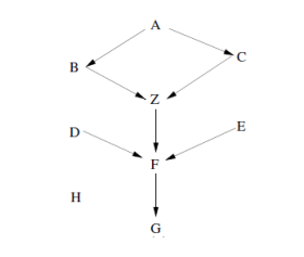
- Given a Bayesian network as in the following figure, what is the Markov Blanket (MB) of node Z?
Info
Hint: Let’s google it
A node’s Markov blanket includes all its parents, children, and children’s parents.
- Download “Example21” dataset. It has the same dependence relationships as the above network
####------III. Finding Markov Blanket of a Node--#####
#Assuming the Example21.csv has been placed in the working directory
data=read.csv("Example21.csv", header=TRUE, sep=",")
head(data)- Learn the MB of Z from data using the IAMB algorithm from bnlearn
# bnlearn requires numeric or factor data types. Convert data of the nine variables (nine columns) in the
# data set to factor data types.
nvar <- ncol(data)
for(i in 1:nvar){data[,i] = as.factor(data[,i]) }

#learn the markov blanket
MB.Z=learn.mb(data, "Z", method="iamb", alpha=0.01)
MB.Z
IV. Estimating causal effect of a variable on another with IDA
Given a Bayesian network, we can estimate the causal effect that a node has on another. In this example, we re-use the dataset d.mat from Section II, and apply ida and idaFast functions from pcalg package to estimate the causal effects.
- Learn the causal structure from data.
#------IV. Estimating causal effect of a variable on another with IDA
# 1. Learn the causal structure from data.
suffStat <- list(C = cor(d.mat), n = nrow(d.mat))
pc.fit <- pc(
    suffStat,
    indepTest = gaussCItest,
    p=ncol(d.mat),
    alpha = 0.01
)
plot(pc.fit@graph)- Estimate the causal effect of node 2 on node 10.
ida(2, 10, cov(d.mat), pc.fit@graph)- Estimate the causal effect of node 4 on nodes 10 and 6.
ida(4, c(10,6), cov(d.mat), pc.fit@graph)
idaFast(4, c(10,6), cov(d.mat), pc.fit@graph)
If the equivalence class contains k DAGs, this will yield k estimated total causal effects.
4. Estimate the causal effect of node 5 on node 7.
ida(5,7, cov(d.mat), pc.fit@graph)
idaFast(5,7, cov(d.mat), pc.fit@graph)- Calculate the causal effect of node 3 on nodes 6, 10.
idaFast(3, c(6,10), cov(d.mat), pc.fit@graph)- Calculate the causal effect of node 2 on node 10 and node 8 on nodes 7, 9.
idaFast(2, 10, cov(d.mat), pc.fit@graph)
idaFast(8, c(7,9), cov(d.mat), pc.fit@graph)
V. Summary of Bayesian Networks
- Generate and draw random DAG with 10 nodes (set seed to 50 and prob to 0.2)
p <- 10
set.seed(50)
myDAG <- randomDAG(p, prob = 0.2)
if (require(Rgraphviz))
{ plot(myDAG, main = "randomDAG(10, prob = 0.2)") }- Generate 10000 samples of the DAG using standard normal error distribution
n <- 10000
mydataset <- rmvDAG(n, myDAG, errDist = "normal")- Use PC algorithm to learn the causal structure of the dataset.
#3. Use PC algorithm to learn the causal structure of the dataset.
suffStat <- list(C = cor(mydataset), n = nrow(mydataset))
my.pc.fit <- pc(
    suffStat,
    indepTest = gaussCItest,
    p=ncol(mydataset),
    alpha = 0.01
)
plot(my.pc.fit@graph)- Estimate the causal effects of node 2 on nodes 5,9.
#4. Estimate the causal effects of node 2 on nodes 5,9.
idaFast(2, c(5,9), cov(mydataset), my.pc.fit@graph)- Find the parent and children set of node 7 using pcSelect (the PC-Simple algorithm)
#5. Find the parent and children set of node 7 using
# pcSelect (the PC-Simple algorithm)
pcS <- pcSelect(dataset[,7],dataset[,-7], alpha = 0.05)
pcS- Find the parent and children set of node 7 using HITON-PC
#6. Find the parent and children set of node 7 using HITON-PC
HITON.PC.7 <- learn.nbr(data.frame(mydataset),"X7", method = "si.hiton.pc", alpha = 0.01)
HITON.PC.7- Learn the Markov blanket of node 7 from data
#7. Learn the Markov blanket of node 7 from data
MB.X7 <- learn.mb(
    data.frame(mydataset),
    "X7",
    method = "iamb",
    alpha = 0.01
)
MB.X7
Note: bnlearn requires the input dataset in dataframe format. Use dataset=data.frame(mydataset) to convert the dataset to dataframe format. Also, check variables names returned after use data.frame
