01.Naïve Bayes Classifier

Haiyue7/31/23About 8 min

Background

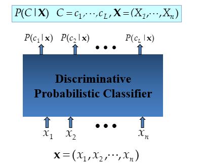
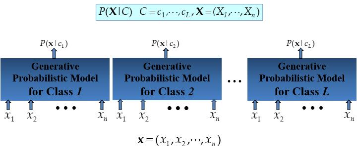
There are three methods to establish a classifier

A. Model a classification rule directly
B. Model the probability of class memberships given input data
C. Make a probabilistic model of data within each class

Examples

Method	discriminative classification	generative classification	probabilistic classification	Examples
A	Yes	No	No	k-NN, decision trees, perceptron, SVM
B	Yes	No	Yes	perceptron with the cross-entropy cost
C	No	Yes	Yes	naive Bayes, model based classifiers

Probability Basics

Prior, conditional and joint probability for random variables

Prior probability: $P (X)$
Conditional probability: $P (X_{1} | X_{2}), P (X_{2} | X_{1})$
Joint probability: $χ = (X_{1}, X_{2}), P (χ) = P (X_{1}, X_{2})$
Relationship: $P (X_{1}, X_{2}) = P (X_{2} | X_{1}) P (X_{1}) = P (X_{1} | X_{2}) P (X_{2})$
Independence: $P (X_{2} | X_{1}) = P (X_{2}) P (X_{1} | X_{2}) = P (X_{1}) P (X_{1}, X_{2}) = P (X_{1}) P (X_{2})$

Bayes Rule (Bayesian Inference)

$P (C | χ) = \frac{P (χ | C) P (C)}{P (χ)}$
$P o s t e r i o r = \frac{L i k e l i h o o d \times P r i o r}{E v i d e n c e}$
$L i k e l i h o o d = P (χ | C)$
$P r i o r = P (C)$
$E v i d e n c e = P (χ)$
$χ$ is what the data we have now.
Basic Idea: We got a data $χ$ , then we want to know the probability of $C$ happened before based what we got ( $χ$ ).

Quiz

We have two six-sided dice. When they are tolled, it could end up with the following occurance:
A. dice 1 lands on side "3"
B. dice 2 lands on side "1"
C. Two dice sum to eight

We set the probabilities:
a. dice 1: $\frac{1}{6}$
b. dice 2: $\frac{1}{6}$
c. dice 3: $\frac{1}{6}$

Answer the following Questions:

$P (A) = P (a | c) = \frac{P (a, c)}{c} = \frac{1}{6}$ .
$P (B) = P (b | a) = \frac{P (a, b)}{a} = \frac{1}{6}$ .
$P (C) = \frac{1}{6} * \frac{1}{6} * 5 = \frac{5}{36}$
$P (A | B) = \frac{P (A, B)}{P (B)} = \frac{1}{6}$
$P (C | A) = \frac{P (A, C)}{P (A)} = \frac{5}{36}$
$P (A, B) = P (A) P (B) = \frac{1}{36}$
$P (A, C) = P (A) P (C) = \frac{1}{6} * \frac{5}{36}$
Is $P (A, C)$ equal to $P (A) * P (C)$ ?
Answer: Yes

Probabilistic Classification

Establishing a probabilistic model for classification

Discriminative model
Generative model

MAP classification rule

MAP: Maximum A Posterior
Assign $x$ to $c^{*}$ if $P (C = c^{*} | \Chi = χ) > P (C = c | \Chi = χ) c \neq c^{*}, c = c_{1}, . . ., c_{_{L}}$

Generative classification with the MAP rule

Apply Bayes rule to convert them into posterior probabilities
$P (C = c_{i} | \Chi = χ) = \frac{P (\Chi = χ | C = c_{i}) P (C = c_{i})}{P (\Chi = χ)} \propto P (\Chi = χ | C = c_{i}) P (C = c_{i})$ for i=1,2,..., L

Naïve Bayes

Bayes classification
$P (C | \Chi) \propto P (\Chi | C) P (C) = P (X_{1}, \cdot \cdot \cdot, X_{n} | C) P (C)$
Difficulty: learning the joint probability $P (X_{1}, \cdot \cdot \cdot, X_{n} | C)$
Naïve Bayes classification
Assumption that all input features are conditionally independent!

\begin{aligned} P (X_{1}, X_{2}, \cdot \cdot \cdot, X_{n} | C) & = P (X_{1} | X_{2}, \cdot \cdot \cdot, X_{n}, C) P (X_{2}, \cdot \cdot \cdot, X_{n} | C) \\ = P (X_{1} | C) P (X_{2}, \cdot \cdot \cdot, X_{n} | C) \\ = P (X_{1} | C) P (X_{2} | C) \cdot \cdot \cdot P (X_{n} | C) \end{aligned}

MAP classification rule: for $x = (x_{1}, x_{2}, \cdot \cdot \cdot, x_{n})$
$[P (x_{1} | C^{*}) \cdot \cdot \cdot P (x_{n} | c^{*})] P (c^{*}) > [P (x_{1} | c) \cdot \cdot \cdot P (x_{n} | c)] P (c), c \neq c^{*}, c = c_{1}, \cdot \cdot \cdot, c_{L}$

Algorithm: Discrete-Valued Features
1. Learning Phase: Given a training set S,
  For each target value of $c_{i} (c_{i} = c_{1}, \cdot \cdot \cdot, c_{_{L}})$
  $\hat{P} (C = c_{i}) \leftarrow$ estimate $P (C = c_{i})$ with examples in S;
  for every feature value $χ_{j k}$ of each feature $X_{j} (j = 1, \cdot \cdot \cdot, n; k = 1, \cdot \cdot \cdot, N_{j})$
  $\hat{P} (X_{j} = x_{j k} | C = c_{j}) \leftarrow$ estimate $P (X_{j} = x_{j k} | C = c_{i})$ with example in $S$ ;
  Output: conditional probability tables; for $X_{j}, N_{j} \times L$ elements
2. Test Phase: Given an unknown instance $\Chi^{^{'}} = (a_{1}^{^{'}}, \cdot \cdot \cdot, a_{n}^{^{'}})$
  Look up tables to assign the label $c^{*}$ to $\Chi^{^{'}}$ if
  $[\hat{P} (a_{1}^{^{'}} | c^{*}) \cdot \cdot \cdot \hat{P} (a_{n}^{^{'}} | c^{*})] \hat{P} (c^{*}) > [\hat{P} (a_{1}^{^{'}} | c) \cdot \cdot \cdot \hat{P} (a_{n}^{^{'}} | c)] \hat{P} (c), c \neq c^{*}, c = c_{1}, \cdot \cdot \cdot, c_{_{L}}$

Examples: Discrete-Valued Features

Original Data

Day	Outlook	Temperature	Humidity	Wind	PlayTennis
D1	Sunny	Hot	High	Weak	No
D2	Sunny	Hot	High	Strong	No
D3	Overcast	Hot	High	Weak	Yes
D4	Rain	Mild	High	Weak	Yes
D5	Rain	Cool	Normal	Weak	Yes
D6	Rain	Cool	Normal	Strong	No
D7	Overcast	Cool	Normal	Strong	Yes
D8	Sunny	Mild	High	Weak	No
D9	Sunny	Cool	Normal	Weak	Yes
D10	Rain	Mild	Normal	Weak	Yes
D11	Sunny	Mild	Normal	Strong	Yes
D12	Overcast	Mild	High	Strong	Yes
D13	Overcast	Hot	Normal	Weak	Yes
D14	Rain	Mild	High	Strong	No

Learning Phase

$P (P l a y = Y e s) = \frac{9}{14}$ $P (P l a y = N o) = \frac{5}{14}$

Outlook	Play = Yes	Play = No
Sunny	$\frac{2}{9}$	$\frac{3}{5}$
Overcast	$\frac{4}{9}$	$\frac{0}{5}$
Rain	$\frac{3}{9}$	$\frac{2}{5}$

Temperature	Play = Yes	Play = No
Hot	$\frac{2}{9}$	$\frac{2}{5}$
Mild	$\frac{4}{9}$	$\frac{2}{5}$
Cool	$\frac{3}{9}$	$\frac{1}{5}$

Outlook	Play = Yes	Play = No
High	$\frac{3}{9}$	$\frac{4}{5}$
Normal	$\frac{6}{9}$	$\frac{1}{5}$

Outlook	Play = Yes	Play = No
Strong	$\frac{3}{9}$	$\frac{3}{5}$
Weak	$\frac{6}{9}$	$\frac{2}{5}$

Test Phase

Given a new instance, predict its label
$x^{'} = (O u t l o o k = S u n n y, T e m p e r a t u r e = C o o l, H u m i d i t y = H i g h, W i n d = S t r o n g)$
Look up tables achieved in the learning phrase
$P (O u t l o o k = S u n n y | P l a y = Y e s) = \frac{2}{9}$
$P (O u t l o o k = S u n n y | P l a y = N o) = \frac{3}{5}$
$P (T e m p e r a t u r e = C o o l | P l a y = Y e s) = \frac{3}{9}$
$P (T e m p e r a t u r e = C o o l | P l a y == N o) = \frac{1}{5}$
$P (H u m i n i t y = H i g h | P l a y = Y e s) = \frac{3}{9}$
$P (H u m i n i t y = H i g h | P l a y = N o) = \frac{4}{5}$
$P (W i n d = S t r o n g | P l a y = Y e s) = \frac{3}{9}$
$P (W i n d = S t r o n g | P l a y = N o) = \frac{3}{5}$
$P (P l a y = Y e s) = \frac{9}{14}$
$P (P l a y = N o) = \frac{5}{14}$
Decision making with the MAP rule
$P (Y e s | x^{'}) : [P (S u n n y | Y e s) P (C o o l | Y e s) P (H i g h | Y e s) P (S t r o n g | Y e s)] P (P l a y = Y e s) = 0.0053$
$P (N o | x^{'}) : [P (S u n n y | N o) P (C o o l | N o) P (H i g h | N o) P (S t r o n g | N o)] P (P l a y = N o) = 0.0206$

Final Result

The fact $P (Y e s | x^{'}) < P (N o | x^{'})$ , we label $x^{'}$ to be “ $N o$ ”.

Algorithm: Continuous-valued Features
- Numberless values for a feature
- Conditional probability often modeled with the normal
  $\hat{P} (X_{j} | C = c_{i}) = \frac{1}{\sqrt{2 π} σ_{j i}} e x p (- \frac{(X_{j} - μ_{j i})^{2}}{2 σ_{j i}^{2}})$
  $μ_{j i}$ : mean (average) of feature values $X_{j}$ of examples for which $C = c_{j}$
  $σ_{j i}$ : standard deviation of feature values $\Chi_{j}$ of examples for which $C = c_{i}$
1. Learning Phase:
  for $\Chi = (X_{1}, \cdot \cdot \cdot, X_{n}), C = c_{1}, \cdot \cdot \cdot, c_{_{L}}$
  Output: $n \times L$ normal distributions and $P (C = c_{i}) i = 1, \cdot \cdot \cdot, L$
2. Test Phase: Given an unknown instance $\Chi^{^{'}} = (a_{1}^{^{'}}, \cdot \cdot \cdot, a_{n}^{^{'}})$
  - Instead of looking-up tables, calculate conditional probabilities with all the normal distributions achieved in the learning phrase
  - Apply the MAP rule to make a decision

Example: Continuous-valued Features

Data

Temperature is naturally of continuous value.
Yes: 25.2, 19.3, 18.5, 21.7, 20.1, 24.3, 22.8, 23.1, 19.8
No: 27.3, 30.1, 17.4, 29.5, 15.1
Estimate mean and variance for each class
$μ = \frac{1}{N} \sum_{n = 1}^{N} x_{n}$
$σ^{2} = \frac{1}{N} \sum_{n = 1}^{N} (x_{n} - σ)^{2}$

According to the formula above, the result could be get
$μ_{y e s} = 21.64, σ_{y e s} = 2.35$
$μ_{N o} = 23.88, σ_{N o} = 7.09$

Learning Phase

output two Gaussian models for P(temp|C)
$\hat{P} (x | Y e s) = \frac{1}{2.35 \sqrt{2 π}} e x p (- \frac{(x - 21.64)^{2}}{2 * {2.35}^{2}}) = \frac{1}{2.35 \sqrt{2 π}} e x p (- \frac{(x - 21.64)^{2}}{11.09})$

$\hat{P} (x | N o) = \frac{1}{7.09 \sqrt{2 π}} e x p (- \frac{(x - 23.88)^{2}}{2 * {7.09}^{2}}) = \frac{1}{7.09 \sqrt{2 π}} e x p (- \frac{(x - 23.88)^{2}}{50.25})$

Relevant Issues

Violation of Independence Assumption
- For many real world tasks, $P (X_{1}, \cdot \cdot \cdot, X_{n} | C) \neq P (X_{1} | C) \cdot \cdot \cdot P (X_{n} | C)$
- Nevertheless, naïve Bayes works surprisingly well anyway!
Zero conditional probability Problem
- If no example contains the attribute value
- In this circumstance, $$ during test
- For a remedy, conditional probabilities estimated with
  $\hat{P} (X_{j} = a_{j k} | C = c_{i}) = \frac{n_{c} + m p}{n + m}$
  $n_{c} :$ number of training examples for which $X_{j} = a_{j k}$ and $C = c_{i}$
  $n :$ number of training examples for which $C = c_{i}$
  $p :$ prior estimate (usually, $p = \frac{1}{t}$ for $t$ possible values os $X_{j}$ )
  $m :$ weight to prior(number of "virtual" examples, $m \geq 1$ )

Summary

Naïve Bayes: the conditional independence assumption
- Training is very easy and fast; just requiring considering each attribute in each class separately
- Test is straightforward; just looking up tables or calculating conditional probabilities with estimated distributions
A popular generative model
- Performance competitive to most of state-of-the-art classifiers even in presence of violating independence assumption
- Many successful applications, e.g., spam mail filtering
- A good candidate of a base learner in ensemble learning
- Apart from classification, naïve Bayes can do more…

Explanation from Thuc

References

Naive Bayes Classifier
Resource from Youtube
Week 2 Slides from Thuc (SP52023)