 Assignment 2
Requirements
Instructions
Requirements Analysis
01.Files Required: ClementsGapWindFarmOutput.xlsx
The tasks for this question are listed below.
- Take the 2011 output (the training set) and find the best ARMA(p,q) model for the data.
- Take the noise
- Calculate
- Find the best ARCH or GARCH model for it.
- Take the developed models for the output and also for the noise and apply them to the 2012 output data.
- Evaluate the performance of the models for one step ahead forecasting with error bounds by calculating the coverage and mean prediction interval width, for both 90% and 95% values.
- Compare the results with constructing the prediction intervals by using the appropriate quantiles.
01.Files Required: MelbourneAirportRain.xlsx
The tasks for this question are listed below.
- Test the months December, January, February, July, August for normality.
- For the months that do not follow a normal distribution, test for a Gamma fit.
- Test December, January, February for correlation, and July, August separately.
- Generate 1000 years of synthetic December, January, February, add the months to get seasonal totals, and generate empirical CDFs for the totals versus the CDFs for the real data.
- Do the same for July, August.
01.Files Required: MtGambierByMonthsTemperature.xlsx
02.Files Required: MtGambierRainfall.xlsx
The tasks for this question are listed below.
- Take the monthly rainfall data from
MtGambierRainfall.xlsxand model the seasonality. Then subtract this from the data. - Use exponential smoothing to see the overall trend in the series - try various values of
αbelow 0.2. - Find the trend for the whole series for the smoothed data, and then find the trends for any sections that you think display differing characteristics.
- Take the data for the month of December and the Annual mean temperature from
MtGambierByMonthsTemperature.xlsxand find the trend over time. - How much has the mean temperature changed over time in each case?
All works below
Question 1
1. Take the 2011 output (the training set) and find the best ARMA(p,q) model for the data.


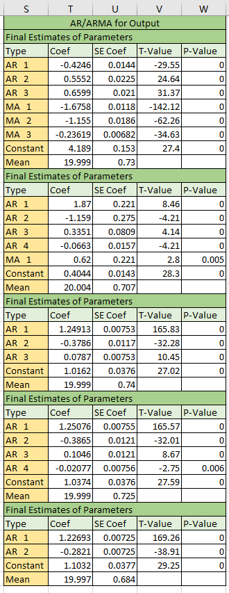
According to the parameters we got. We should compare the mean of squared error (MSE) and p-value of the parameters for each model to select a proper model, the smaller the better. The table below lists all the MSEs.
| ARMA(3,3) | ARMA(4,1) | AR(4) | AR(3) | AR(2) | |
|---|---|---|---|---|---|
| mean of square error | overflow | 85.89976922 | 24.75701538 | 24.76769416 | 24.92197907 |
According to the mean of square error, the performance of AR(3) and AR(4) are similar, I select the AR(4) as the best model.
2. Take the noise
I could get the residuals based on the model AR(4) get from the previous step, and name the residuals as Zt-AR(4). Then, we could see the SACF according to the ACF and PACF, like the pictures below.


According to the result from ACF and PACF, the Zt-AR(4) is not suit for using ARMA model to forecast.
3. Calculate
For calculating the ARCH effect, it should be seperated into two parts, one for ARCH model, another for GARCH model.
3.1 Effect for ARCH model


According to the SACF above, there is ARCH effect for ARCH model.
3.2 Effect for GARCH model


According to the SACF above, there is also ARCH effect for GARCH model.
4. Find the best ARCH or GARCH model for it.
For this part, I try to find all possible ARCH and GARCH models, then try to compare the results for finalizing the model.
4.1 ARCH model
According to the squared residuals for ARCH model, five AR models for the dataset could be found, the parameters like the picture below.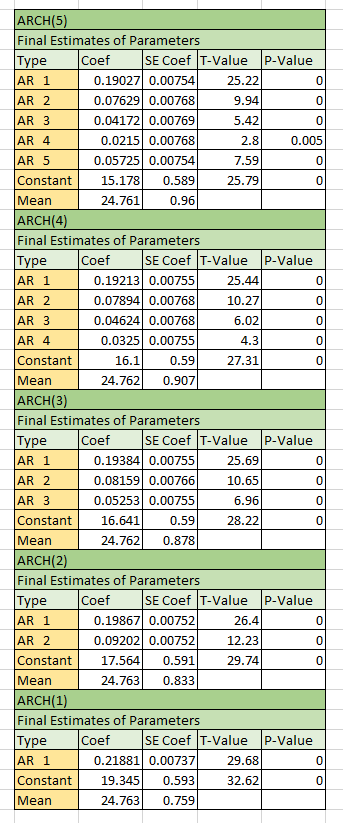
According to the parameters above, the coverage rate could be calculated like the picture below.
According to the result, all the coverage rate for the five model are similar, and they all approach 89.6% for score 1.96.
4.2 GARCH model
According to the squared residuals for GARCH model, 10 ARMA model for the dataset could be found, the parameters like the picture below.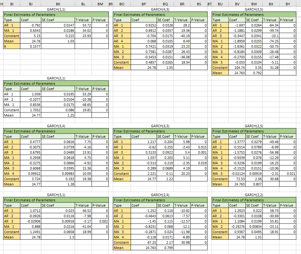
For some models will occurs negative values, which will lead to the specified model unavaliable. The coverage rate for each model like the picture below.
According to the result the best model for the residuals is GARCH(1,1), the coverage could be 99.15%.
5. Take the developed models for the output and also for the noise and apply them to the 2012 output data.
According to previous steps, we got two models for the dataset. One is AR(4), another one is GARCH(1,1). All the models will apply to 2012 dataset. The result like the picture below.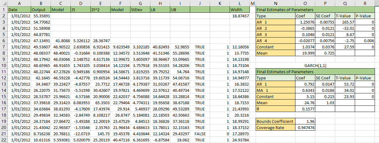
6. Evaluate the performance of the models for one step ahead forecasting with error bounds by calculating the coverage and mean prediction interval width, for both 90% and 95% values.
The score of 90% is about 1.65 and the score of 95% is about 1.96. The 95% result like the picture below.
The 95% coverage result like the picture below.
The 90% coverage result like the picture below.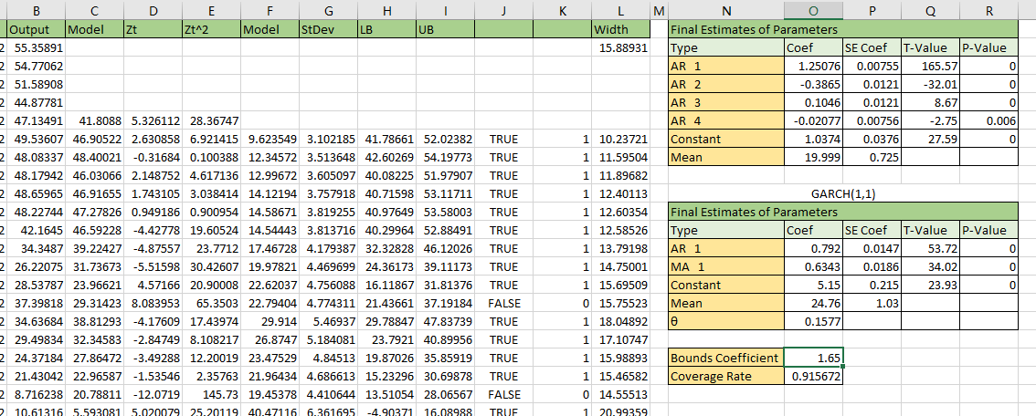
The statistical summary for the residuals of 2012 data like the picture below.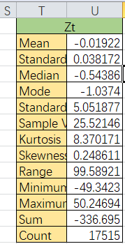
According to the statistical summary, the standard deviation is about 5.05. The mean predictiion interval width of 95% coverage is about 18.87, for 90% coverage is about 15.89. The real coverage with 1.96 score is 94.75%, and 91.57% for 1.65 score. So we could get
The mean of prediction interval for 90% coverage is 15.88931, and 18.87457 for 90% coverage.
The results suggest that the model is quiet well for the dataset.
7. Compare the results with constructing the prediction intervals by using the appropriate quantiles.
The picture below is the prediction interval using GARCH and quantile method.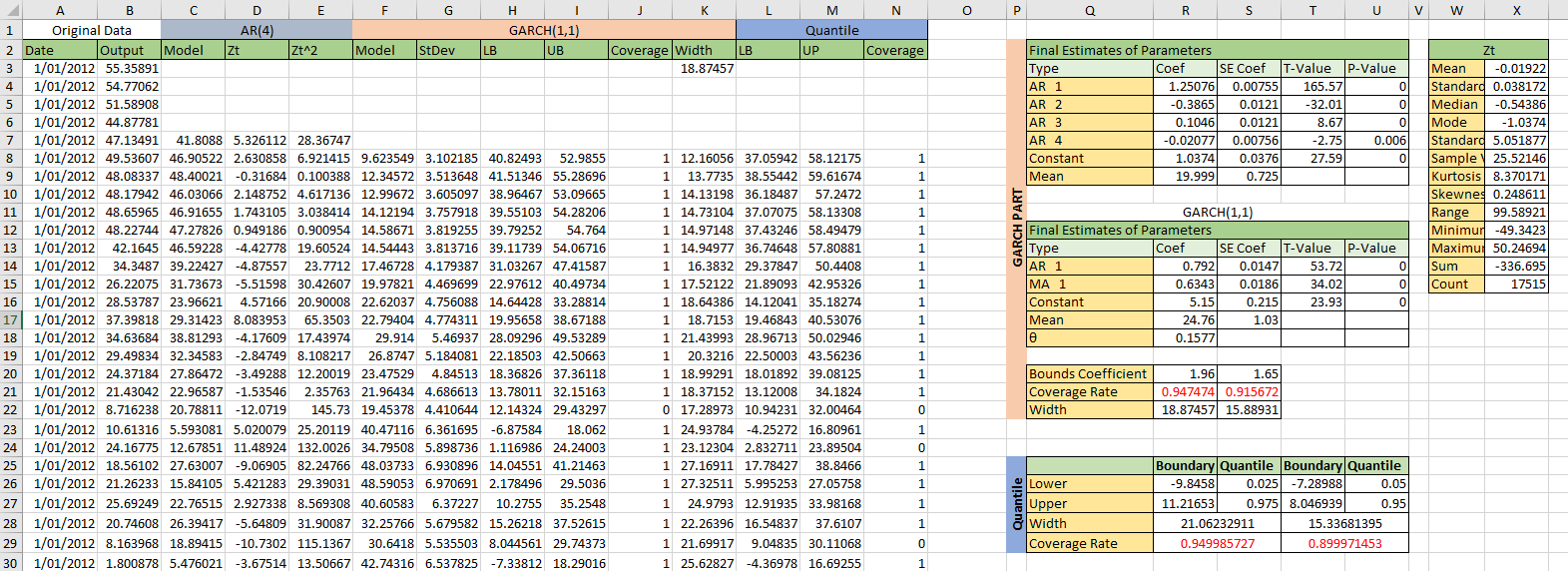
The picture below is the result of quantile approach and GARCH.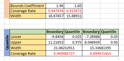
According to the result ...
A simple technique to estimate prediction intervals for any regression model
Question 2
The tasks for this question are listed below.
1. Test the months December, January, February, July, August for normality.
For normality test, the ppplot and histogram could be used for testing.
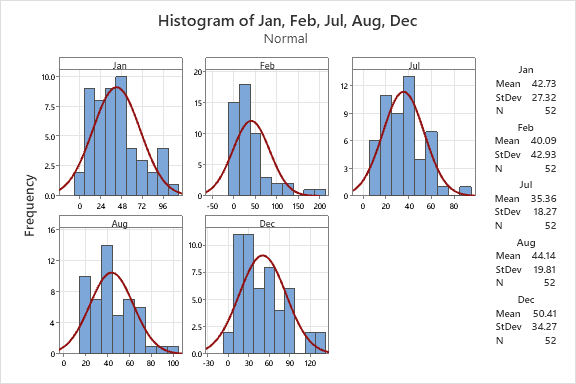
According to the histogram all the distribution of the months are right skewed.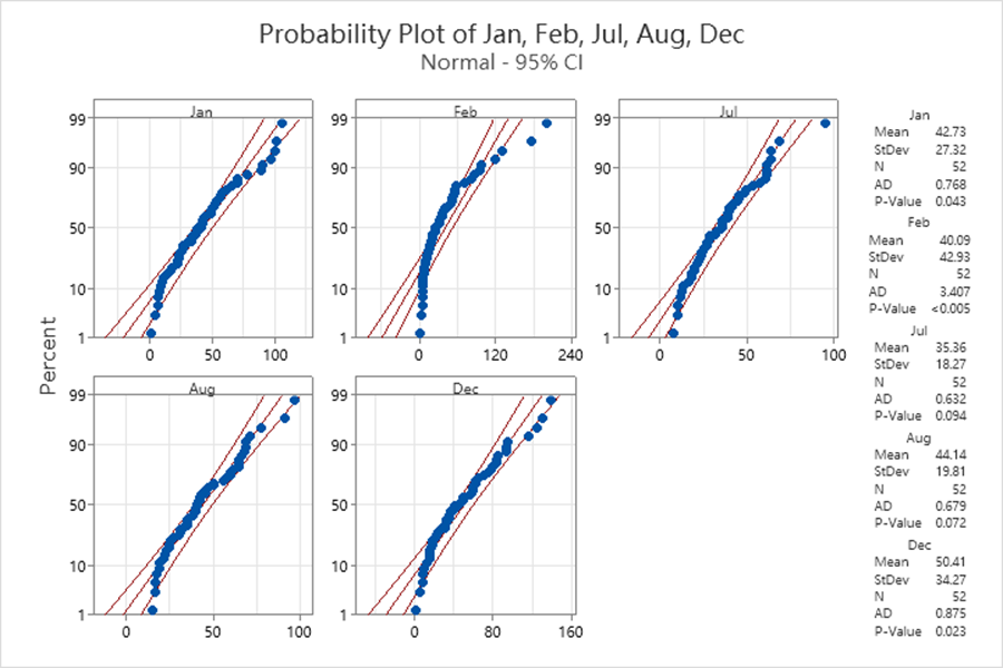
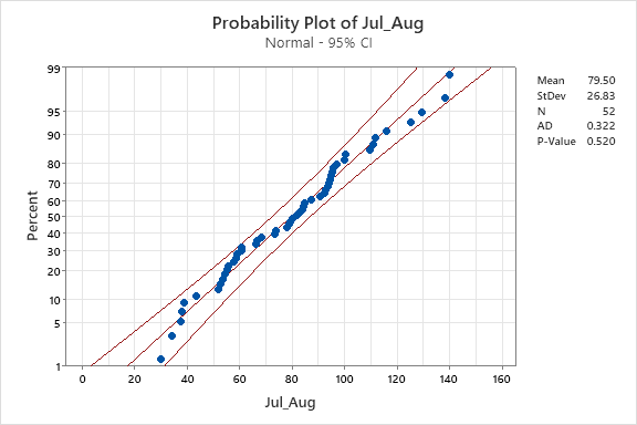
According to the ppplot result, the p-value of July and August is greater than 0.05, we can not reject they follow the normal distribution, on the other hand the p-value of January February and December is less than 0.05, we reject the datasets of the three months follow normal distribution.
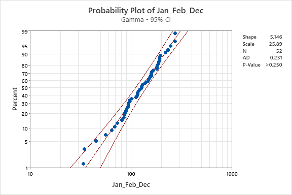
2. For the months that do not follow a normal distribution, test for a Gamma fit.
There are two steps for this question. The first step is to calculate the
2.1 Get the parameters for gamma
The parameters 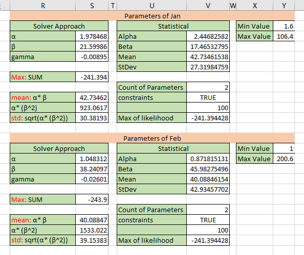
2.2 Visulize the distribution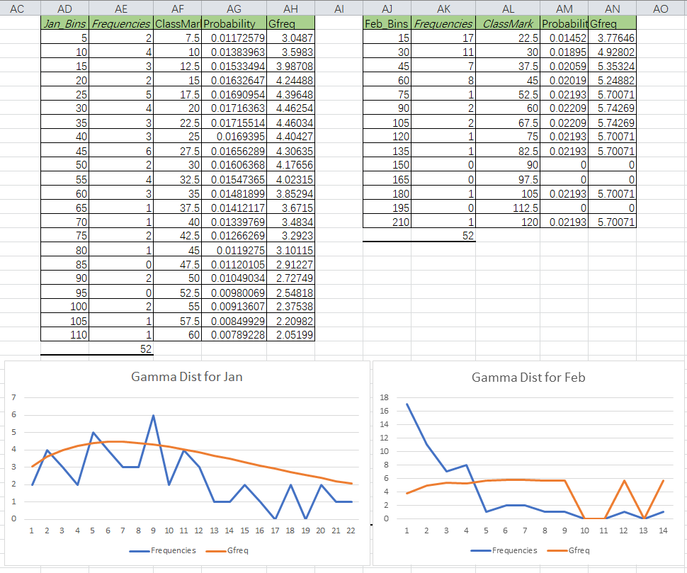
2.1 Get the parameters for gamma
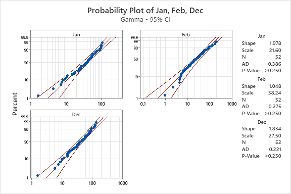
2.2 Visualization


3. Test December, January, February for correlation, and July, August separately.
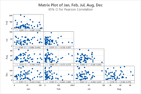
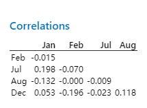
Correlations matrix
| Jan | Feb | Jul | Aug | |
|---|---|---|---|---|
| Feb | -0.015 | |||
| Jul | 0.198 | -0.070 | ||
| Aug | -0.132 | -0.000 | -0.009 | |
| Dec | 0.053 | -0.196 | -0.023 | 0.118 |
According to the correlation matrix, there is almost no correlation among the months.
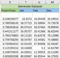
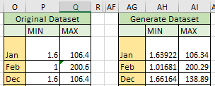
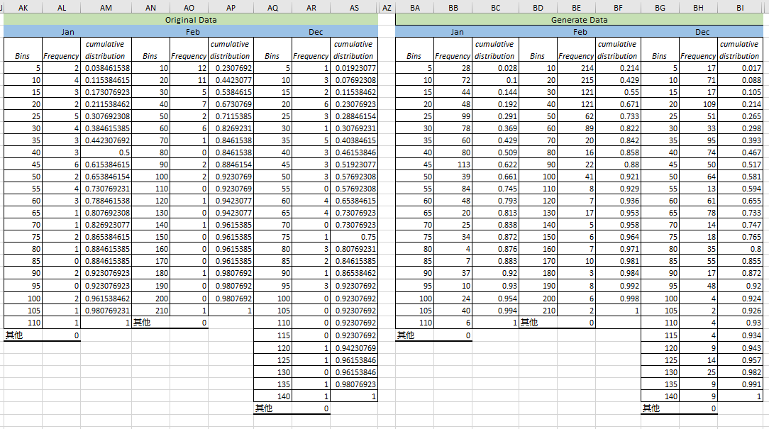
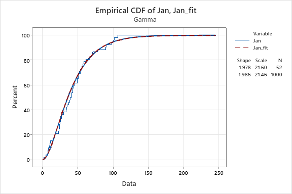
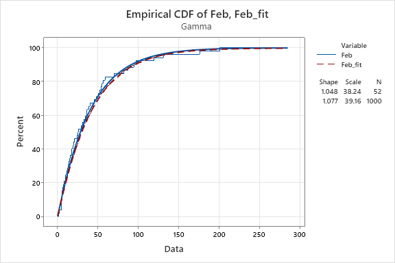
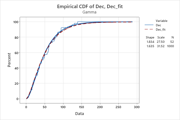
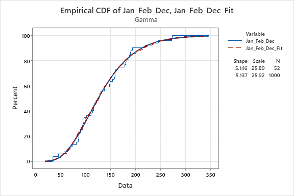
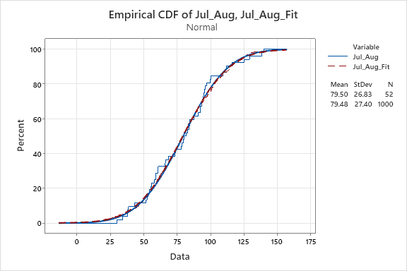
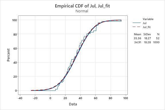
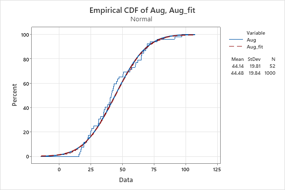
4. Generate 1000 years of synthetic December, January, February, add the months to get seasonal totals, and generate empirical CDFs for the totals versus the CDFs for the real data.


5. Do the same for July, August.
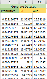
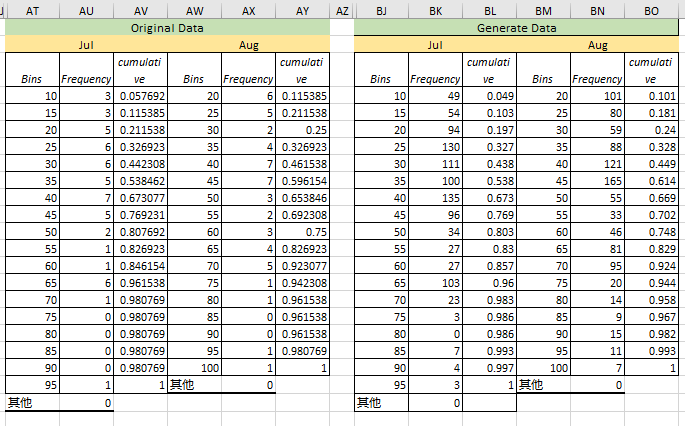
Because of July, August perhaps follow normal distribution, here we should generate normal distribution synthetic data.



Question 3
The tasks for this question are listed below.
1. Take the monthly rainfall data from MtGambierRainfall.xlsx and model the seasonality. Then subtract this from the data.
There are three steps for this question. The first step is to find the best frequencies, the second step is to find the proper parameters for seasonalities, and the last step is to visualize the seasonality result.
The picture below is the frequencies for the dataset. The 50 and 550 is the best for the dataset.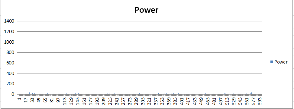
The picture below is the seasonality parameters using the frequencies got from step1. And also we got the final model and the residuals.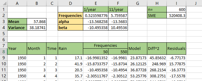
The picture is the visualization for the final model of seasonality.
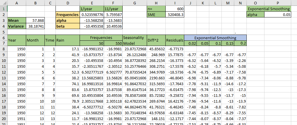
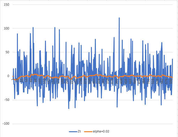
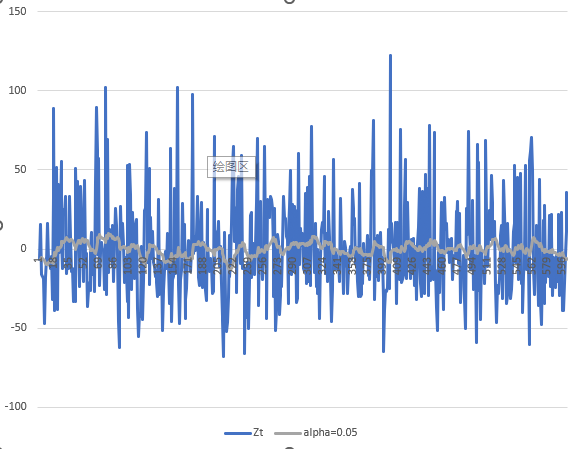
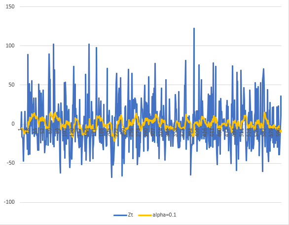
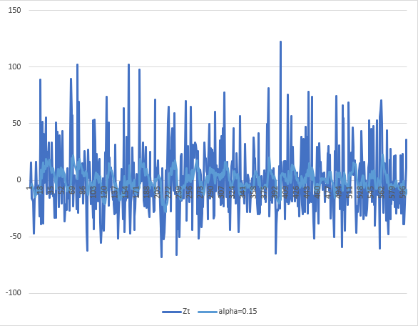
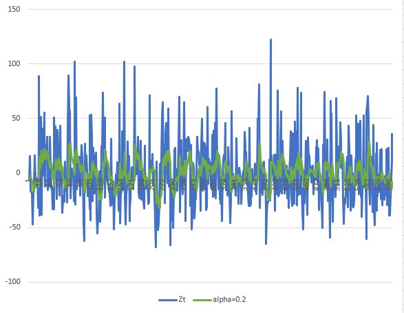
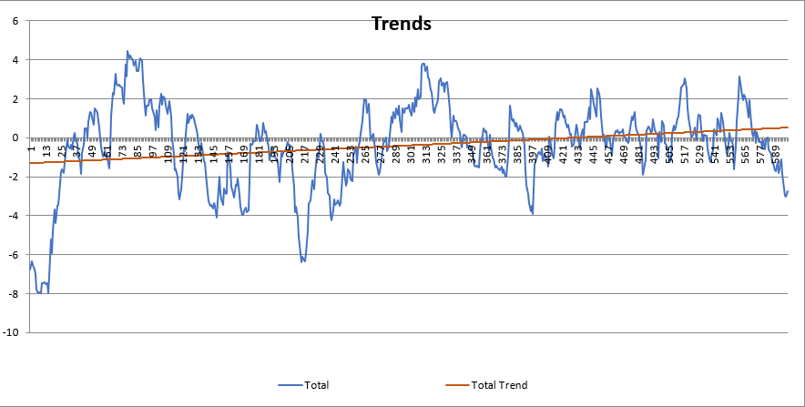
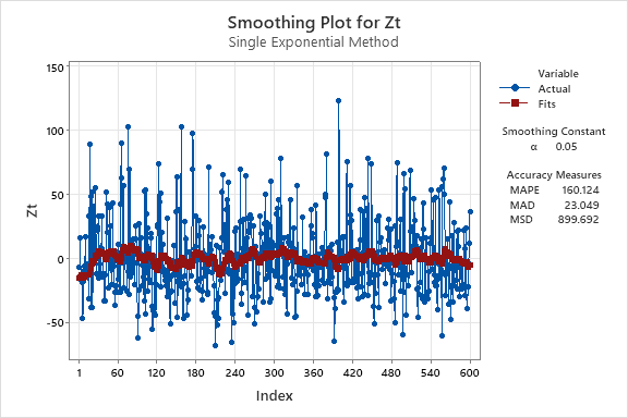
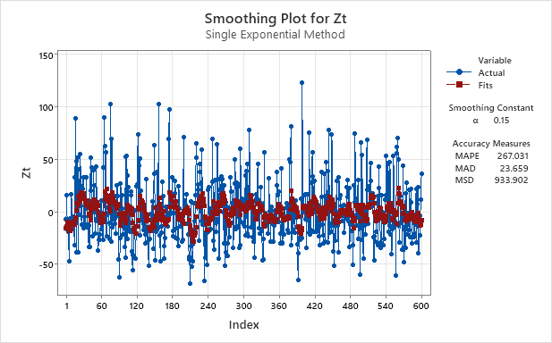
2. Use exponential smoothing to see the overall trend in the series - try various values of α below 0.2.
For this question, I will show the results of four values for the


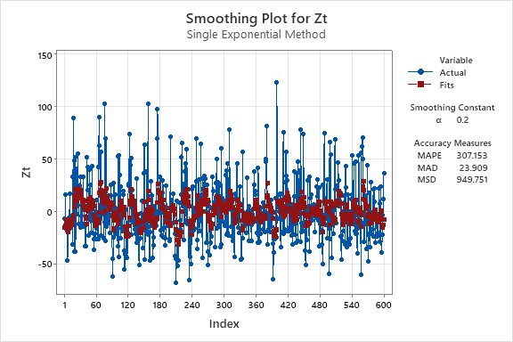
3. Find the trend for the whole series for the smoothed data, and then find the trends for any sections that you think display differing characteristics.
I will set the parameter
3.1 Find the trend of whole dataset.
I use the univariate linear regression to model the trend. The result like the picture below.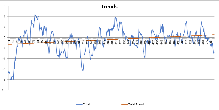
3.2 Split whole dataset into multiple sections.
Accoriding the visualization of the dataset, the dataset could be split into two sections, the first section(from the begining to 60) rise rapidly, and the second section oscillate around a variable. So the dataset could be split into two sections like the pciture below.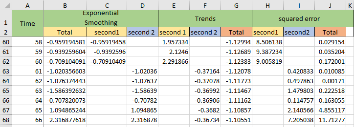
3.3 find the trends for the two sections
The trends of the two sections like the picture belowl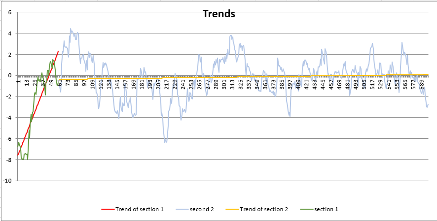
4. Take the data for the month of December and the Annual mean temperature from MtGambierByMonthsTemperature.xlsx and find the trend over time.
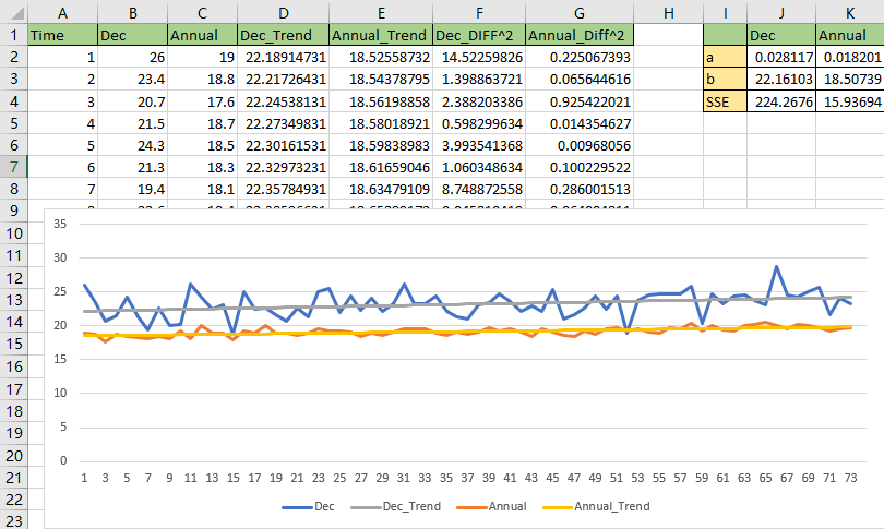
5. How much has the mean temperature changed over time in each case?
According to the result from the last step, the mean temperature changed over time should be calculated via the linear regression parameters with the whole 73 years on this dataset.
The temperature changed over time for December should be,
a * year = 0.028117 * 73 = 2.05
The temperature changed over time for December should be,
a * year = 0.018201 * 73 = 1.32
