 Assignment 1
Requirements
Instructions
Instructions
Requirements Analysis
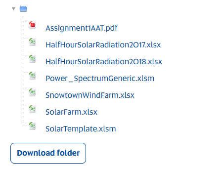
For this question you will need the files from the website named
a. HalfHourSolarRadiation2017.xlsxb. HalfHourSolarRadiation2018.xlsxc. PowerSpectrumGeneric.xlsmd. SolarTemplate.xlsmThe tasks for this question are listed below.
- Take the solar radiation data from File
a, and copy it into Filec, and run the power spectrum tool to find out which frequencies are important. - Use File
cto find the Fourier series model for the seasonality.Info
Note that the Template is designed for hourly data. You will have to make some adjustments to use it for half hourly data plus change the relevant frequencies if necessary.
- Take the difference between the data and the Fourier model - the residuals - and take them to Minitab and find the best ARMA(p,q) model.
- Use the ARMA model to forecast one step ahead for the residuals and add that to the Fourier series model to get the full one step ahead forecast.
- Use the error metrics defined below to evaluate the model.
- Use the models you have developed for 2017 to see how they perform for the 2018 data, the out of sample data. Comment on the differences in the error metrics.
The Normalised Mean Bias Error (NMBE) is defined by taking the difference between the data
Tips
Note that for solar radiation, we only do the calculation for solar elevation greater than or equal to 10 degrees. That is why I included the elevation data.
We also define the Normalised Mean Absolute Error (NMAE)
- Take the solar radiation data from File
For this question you will need the files
a. SolarFarm.xlsxb. PowerSpectrumGeneric.xlsmc. SolarTemplate.xlsmIn File
ais solar farm output in MegaWatts(MW) for every five minutes for a year.- You are to use the power spectrum to decide on the necessary frequencies, and
- then alter the File
cto find the Fourier series model. - Then calculate the residuals and find their ARMA model.
- Then calculate the one step ahead forecast and evaluate the error metrics for all values of output greater than zero.
The file on the website SnowtownWindFarm.xlsx has a one year of half hour output from a wind farm in South Australia.
- Use the power spectrum file from above to show that there is no significant seasonality in the data.
- You are now to Compare the best
AR(p)model with the bestARMA(p,q)model that you can find. Use the error metrics for your comparison. - Is there a difference in the number of parameters to estimate in the two models? If so, is it worth it to use the one with extra parameters?
All works below
Question 1
The GHI column is selected as the target variable. Because of the data is half hourly dataset, it's a lots of data and not easy to use for analysis. So I convert it into daily data.
Taks1: Getting Frequencies
- DFT
Usingpowerspectrumexcel to get the best frequencies.Info
Step1: using half-hourly data
Step2: Number of data: 17520, Number of frequencies: 2000

It could easily be found that the power of frequencies is greater than 500. Then we could select the value like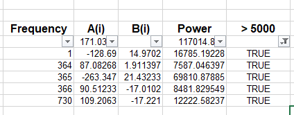
- Results
Results
The best frequencies are [1, 364,365, 366, 730].
Task2: Getting the fourier model
- Seasonality
We could calculate the coefficients for the seasonality using fourier model.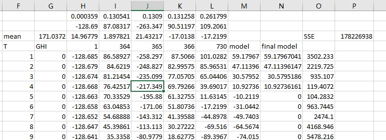
The parameters like below:
P3 = SUM(O5:O17524)
G3 = AVERAGE(G5:G17524)

H1 = 2*PI()/17520*H$4
I1 = 2*PI()/17520*I$4
J1 = 2*PI()/17520*J$4
K1 = 2*PI()/17520*K$4
L1 = 2*PI()/17520*L$4

'The formula should be drag down for filling the necessary cells
H5 = H$2*COS(H$1*$F5)+H$3*SIN(H$1*$F5)
I5 = I$2*COS(I$1*$F5)+I$3*SIN(I$1*$F5)
J5 = J$2*COS(J$1*$F5)+J$3*SIN(J$1*$F5)
K5 = K$2*COS(K$1*$F5)+K$3*SIN(K$1*$F5)
L5 = L$2*COS(L$1*$F5)+L$3*SIN(L$1*$F5)

M5 = SUM(H5:L5)+$G$3
O5 = (G5-M5)^2
We should use the solver to minimize the target function in P3

We could see the seasonality results

Task 3: Getting the coefficients for AR model
Now we got residuals
The formula of residuals
O5 = G5-M5Then copy all the residuals to minitab for autocorrelation analysis.
Auto Corrrelation Result

Partial Auto Corrrelation Result

According to the results of Auto correlation and Partial Auto Correlation, it can see the values are correlated with the past values.
Now we try to use the ARIMA to find the coefficients of the forcasting model.
The first step we try to set the autoregressive is 5.

The results are here.

We could see the pvalue of AR5 and Constant are more then 0.05, so we need the exclude the constant and decrease the number of lags, now we try to set autoregressive is 4.

According to the results we could see all the pvalues are less than 0.05, so we could use AR(4) model to model the residuals.
Task 4: Using the ARMA model to forecast
Now we copy the coefficients to excel, and try to model the AR(4) like the picture below..png)
S9 = Q8*$V$5 + Q7*$V$6 + Q6*$V$7 + Q5*$V$8We could to visualize the fitting result of AR(4)
Partial Fitting Resultpartialfittingresult.png)
Whole Data Fitting Resultwholefittingresult.png)
According to the results above, we could know, the seasonality and AR(4) could fitting very well on our data. Now we need to combine the two components to see the final result.

AA9 = M9+S9Partial Final Model Fitting Result
Whole Final Model Fitting Result
According to the graph, we could know the final model could fit the data very well.
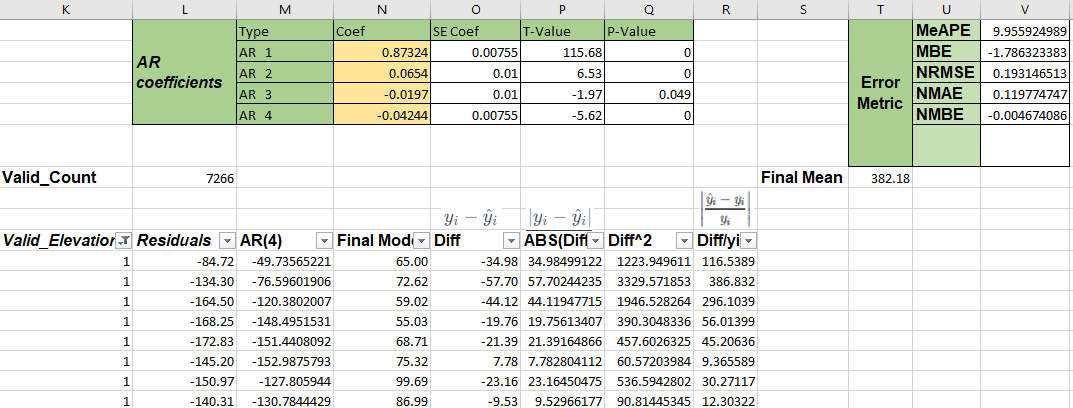
Task 5: To evaluating the model
I switch to template excel to implement all the steps. So, the postion for cells will totally change. You could change all values above to the correct position.
We could know the error metric include several indicators.
- indicators
Formulas
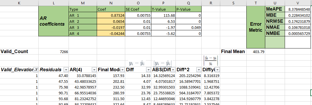
L7 = SUBTOTAL(2,K15:K17530)
T7 = SUBTOTAL(1,N15:N17530)
V1 = AGGREGATE(12,1,R15:R17530)
V2 = SUBTOTAL(109, O15:O17530)/L7
V3 = SQRT(SUBTOTAL(109,Q15:Q17530)/L7)/T7
V4 = SUBTOTAL(109, P15:P17530)/(L7*T7)
V5 = SUBTOTAL(109, O15:O17530)/(L7*T7)

# H column are the data of elevations
K1  = IF(H11>=10,1,0)

O15 = (A15-N15)
P15 = ABS(O15)
Q15 = O15^2
R15 = IF(A15=0,0,ABS(K15*P15/A15)*100)
If we want to select the valid metric according to our data, should filter all the data where K column equals 1.
Then we get.
Task 6: Testing the ARMA model using 2018 data
Using the model get from the 2017 dataset, to predict the data in 2018.
The whole fitting result
The part fitting result
Actually, when the data if not possible be zero, so we could reset all negative number to 0. so we could get.
- Important Node
Important
Some steps above does not use the template file, it's a little ugly and unclear. I will redo it in the solar template, the files could download via the like below.
All code please read the content on Power Spectrum
- All python codeloading libraries
import math
import pandas as pd
import requests as req
import numpy as np
import matplotlib.pyplot as plt
DFT & Plotdef DFT_Excel(data, num_frequencies): num_data = len(data) n2 = num_data / 2 ret = {'frequency':[], 'ai':[], 'bi':[], 'power':[]} for i in range(num_frequencies): s1 = 0 s2 = 0 s0 = sum(data) for j in range(1, num_data): cit = math.cos(math.pi * i / n2*(j+1)) sit = math.sin(math.pi * i / n2*(j+1)) s1 = s1 + cit * data[j] s2 = s2 + sit * data[j] s1 /= n2 s2 /= n2 ret['frequency'].append(i) ret['ai'].append(s1) ret['bi'].append(s2) ret['power'].append(s1**2 + s2**2) ret['ai'][0] = sum(data)/len(data) return pd.DataFrame(ret) def dft_plot(power_spectrum, title): plt.bar(daily_power_spectrum['frequency'][1:], daily_power_spectrum['power'][1:],) plt.title(title, fontsize=14) plt.xlabel('Frequency', fontsize=14) plt.ylabel('Power', fontsize=14) #plt.grid(True) plt.show()Reading dataresponse = req.get('https://seamice.github.io/data/unisa/AdvancedAnalytic1/assignment1/ HalfHourSolarRadiation2017.xlsx') solar_radia2017 = pd.read_excel(response.content)PowerSpectrum# convert half-hourly data to daily data solar_radia2017['group'] = solar_radia2017.index / 2 solar_radia2017['group'] = solar_radia2017['group'].apply(math.floor) hourly_data = solar_radia2017.groupby('group').sum() hourly_power_spectrum = DFT_Excel(hourly_data.GHI, 200) dft_plot(hourly_power_spectrum, 'Hourly Power Spectrum')
Using Power Spectrum method to get the frequencies graph like below.

According to the frequency graph, it's easy to find the best frequency is 1.
Question 2
Task 1: Find frequencies
Copy data from solarfarm to powerspectrum, using Number of objects: 105120, number of frequencies: 10000. We could see the power barchart like below.

According to the graph above, we could know the best frequencies is around 10, here we regards the frequencies that the value of power are greater than 2, the best frequencies could get like the picture below.
Task 2: Make seasonality
After getting the best frequencies, we could using solver to minimize the SSE(Sum square of error), to find the best coefficients to our model.


We could visualize the seasonality model fitting resutls.


According to the graph, we could see the seasonality could fit the data well, but still have a large gap in the middle of the data.
Task 3: ARIMA coefficients
After getting the seasonality model, then could get the residuals to find the cofficients for ARIMA model.
The autocorrelation result

The partial autocorrelation result

According to the data graph, we could find the data the correlated with the past data. Next we try to find the best coefficients for the forecasting model.

According to the graph above, we could know the constant is no significant with the model, so we should remove it during searching the coefficients.

After getting the coefficients, we could using the model to forecast the data, the pictures below show the forecasting results.MA(1)FittingResult.png)
MA(1)FittingResult.png)
Task 4: Final model
The previous has been split the data analysis into two components, in this step, combine the two components to form the final model.
The picture below will show the final results.

Task 5: Error Metric
According to the source data, which contains zero value, so the MeAPE is not suit for evaluating the forecasting model.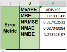
Question 3
Task 1: Find frequencies
When we use the power spectrum, the result should get like
According to the graph above, it not easy to find the few frequencies that holds the important position. It seems there is lots of frequencies that are important. So, we could say there is no significant seasonality in the data.
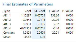
Task 2: Compare AR(p) and ARMA(p,q)
According to the previous results, we just need to find the coefficients for AR(p) and ARMA(p,q) model on the original dataset.
After searching, the best AR model should be AR(4), and ARMA model should be ARMA(2,1).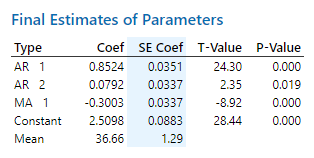


WholeFittingResult.png)
PartialFittingResult.png)

Download the solarRadiation Process
The final Excel
final Report

